Location of income tax offices

The example description in the following section is taken from Section 15.5 Location of income tax offices of the book Applications of optimization with Xpress-MP. The income tax administration is planning to restructure the network of income tax offices in a region. The number of inhabitants of every city and the distances between each pair of cities are known (see table below). The income tax administration has determined that offices should be established in three cities to provide sufficient coverage. Where should these offices be located to minimize the average distance per inhabitant to the closest income tax office ?

	1	2	3	4	5	6	7	8	9	10	11	12
1	0	15	37	55	24	60	18	33	48	40	58	67
2	15	0	22	40	38	52	33	48	42	55	61	61
3	37	22	0	18	16	30	43	28	20	58	39	39
4	55	40	18	0	34	12	61	46	24	62	43	34
5	24	38	16	34	0	36	27	12	24	49	37	43
6	60	52	30	12	36	0	57	42	12	50	31	22
7	18	33	43	61	27	57	0	15	45	22	40	61
8	33	48	28	46	12	42	15	0	30	37	25	46
9	48	42	20	24	24	12	45	30	0	38	19	19
10	40	55	58	62	49	50	22	37	38	0	19	40
11	58	61	39	43	37	31	40	25	19	19	0	21
12	67	61	39	34	43	22	61	46	19	40	21	0
Pop. (in 1000)	15	10	12	18	5	24	11	16	13	22	19	20

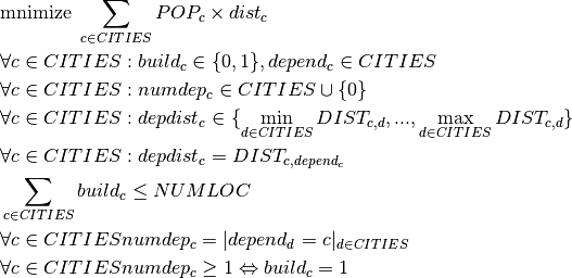
Model formulation

Let be the set of cities. For the formulation of the problem, two groups of decision variables are necessary: a variable that is one if and only if a tax office is established in city , and a variable that takes the number of the office on which city depends. For the formulation of the constraints, we further introduce two sets of auxiliary variables: , the distance from city to the office indicated by , and , the number of cities depending on an office location.

The following relations are required to link the with the variables:

• counts the number of occurrences of office location among the variables dependc;

• if and only if the office in is built (as a consequence, if the office in is not built, then we must have );

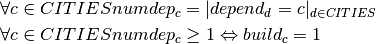
Since the number of offices built is limited by the given bound , i.e. , it would actually be sufficient to formulate the second relation between the and variables as the implication If then the office in must be built, and inversely, if the office in is not built, then we must have .

The objective function to be minimized is the total distance weighted by the number of inhabitants of the cities. We need to divide the resulting value by the total population of the region to obtain the average distance per inhabitant to the closest income tax office. The distance from city to the closest tax office location is obtained by a discrete function, namely the row of the distance matrix indexed by the value of :

Implementation

To solve this problem, we define a branching strategy with two parts, one for the variables and a second strategy for the variables. The latter are enumerated using the KSplitDomain branching scheme that divides the domain of the branching variable into several disjoint subsets (instead of assigning a value to the variable). We now pass an array of type KBranchingSchemeArray as the argument to the constructor of KSolver. The different strategies will be applied in their order in this array. Since our enumeration strategy does not explicitly include all decision variables of the problem, Artelys Kalis will enumerate these using the default strategy if any unassigned variables remain after the application of our search strategy.

C++PythonJava

// Number of cities
int NC = 12;
// Distance matrix
int DIST[12][12];
// Population of cities
int POP[12] = {15, 10, 12 ,18 ,5 ,24, 11, 16, 13, 22, 19 ,20};
// Desired number of tax offices
int NUMLOC = 3;
// 1 if office in city, 0 otherwise
KIntVarArray build;
// Office on which city depends
KIntVarArray depend;
// Distance to tax office
KIntVarArray depdist;
// Number of depending cities per off.
KIntVarArray numdep;
// Objective function variable
KIntVar * totDist;

// Creation of the problem in this session
KProblem problem(session,"J-5 Tax office location");

// index variables
int b,c,d;

// Calculate the distance matrix
// Initialize all distance labels with a sufficiently large value
for (c=0;c<NC;c++) {
    for (d=0;d<NC;d++) {
        DIST[c][d] = MAX_INT;
    }
}
// Set values on the diagonal to 0
for (c=0;c<NC;c++) {
    DIST[c][c] = 0;
}

// Length of existing road connections
DIST[0][1] = 15;DIST[0][4] = 24;DIST[0][6] = 18;DIST[1][2] = 22;
DIST[2][3] = 18;DIST[2][4] = 16;DIST[2][8] = 20;DIST[3][5] = 12;
DIST[4][7] = 12;DIST[4][8] = 24;DIST[5][8] = 12;DIST[5][11] = 22;
DIST[6][7] = 15;DIST[6][9] = 22;DIST[7][8] = 30;DIST[7][10] = 25;
DIST[8][10] = 19;DIST[8][11] = 19;DIST[9][10] = 19;DIST[10][11] = 21;

// distances are symetric
for (b=0;b<NC;b++) {
    for (c=0;c<NC;c++) {
        if (DIST[b][c] != MAX_INT) {
            DIST[c][b] = DIST[b][c];
        }
    }
}

// Update shortest distance for every node triple
for (b=0;b<NC;b++) {
    for (c=0;c<NC;c++) {
        for (d=0;d<NC;d++) {
            if (c<d) {
                if (DIST[c][d] > DIST[c][b]+DIST[b][d]) {
                        DIST[c][d] = DIST[c][b]+DIST[b][d];
                        DIST[d][c] = DIST[c][b]+DIST[b][d];
                }
            }
        }
    }
}
// total popuplation
int sumPop=0;
char name[80];

// building variables
for (c=0;c<NC;c++) {
    sprintf(name,"build(%i)",c);
    build += (* new KIntVar(problem,name,0,1) );

    sprintf(name,"depend(%i)",c);
    depend += (* new KIntVar(problem,name,0,NC-1) );

    int dmin=DIST[c][0];
    int dmax=DIST[c][0];
    int d;
    for (d=1;d<NC;d++) {
        if (DIST[d][c] < dmin) {
            dmin = DIST[c][d];
        }
        if (DIST[c][d] > dmax) {
            dmax = DIST[c][d];
        }
    }
    sprintf(name,"depdist(%i)",c);
    depdist += (* new KIntVar(problem,name,dmin,dmax) );

    sprintf(name,"numdep(%i)",c);
    numdep += (* new KIntVar(problem,name,0,NC) );

    // compute total popuplation for solution printing routines
    sumPop += POP[c];

}

// Distance from cities to tax offices
for (c=0;c<NC;c++) {
    // Auxiliary array used in constr. def.
    KIntArray D;
    for (d=0;d<NC;d++) {
        D += DIST[d][c];
    }
    KEltTerm kelt(D,depend[c]);
    problem.post(kelt == depdist[c]);
}

// Number of cities depending on every office
for (c=0;c<NC;c++) {
    KOccurTerm koc(c,depend);
    problem.post(koc == numdep[c]);
}

// Relations between dependencies and offices built
for (c=0;c<NC;c++) {
    problem.post(KEquiv(build[c] == 1, numdep[c] >= 1));
}

// Limit total number of offices
KLinTerm sbuild;
for (c=0;c<NC;c++) {
    sbuild = sbuild + build[c];
}
problem.post(sbuild <= NUMLOC);

// Objective: weighted total distance
totDist = new KIntVar(problem,"totdDist",0,10000);
KLinTerm popDistTerm;
for (c=0;c<NC;c++) {
    popDistTerm = popDistTerm + POP[c] * depdist[c];
}
problem.post(popDistTerm == *totDist);

// propagating problem
if (problem.propagate()) {
    printf("Problem is infeasible\n");
    exit(1);
}

problem.setObjective(*totDist);
problem.setSense(KProblem::Minimize);

// Search strategy
KBranchingSchemeArray myBa;
myBa += KAssignAndForbid(KMaxDegree(),KMaxToMin(),build);
myBa += KSplitDomain(KSmallestDomain(),KMinToMax(),depdist,true,5);

// creation of the solver
KSolver solver(problem,myBa);

// Solve the problem
if (solver.optimize())  {
    KSolution * sol = &problem.getSolution();
    // do something with optimal solution
}

int totalDist = problem.getSolution().getValue(*totDist);
// Solution printing
printf("Total weighted distance: %d (average per inhabitant: %f\n", totalDist,totalDist / (float)sumPop);
for (c=0;c<NC;c++) {
    if (problem.getSolution().getValue(build[c]) > 0) {
        printf("Office in %i: ",c);
        for (d=0;d<NC;d++) {
            if (problem.getSolution().getValue(depend[d]) == c) {
                printf(" %i",d);
            }
        }
        printf("\n");

    }
}

Results

The optimal solution to this problem has a total weighted distance of 2438. Since the region has a total of 185,000 inhabitants, the average distance per inhabitant is 2438/185 13.178 km. The three offices are established at nodes 1, 6, and 11. The first serves cities 1, 2, 5, 7, the office in node 6 cities 3, 4, 6, 9, and the office in node 11 cities 8, 10, 11, 12.