Continuous variables and numerical CSP
In this section, you will find all relevant information to solve numerical constraint satisfaction problem with Artelys Kalis. This includes:
how to create numerical decision variables ;
how to constrain numerical and integer decisions variables ;
how to solve a simple numerical CSP
All features are going to be illustrated by a simple intersection problem.
Finding the intersections of two circles
Consider the following problem: given two circles of same radius (the first circle centered on the origin and the second on the point of coordinates  ), find the cartesian coordinates of
all the intersection points of the two circles such that the radius is a natural number belonging to the interval
), find the cartesian coordinates of
all the intersection points of the two circles such that the radius is a natural number belonging to the interval ![[0..4]](_images/math/07f5b4294cae0b4efcbc176376005a6221aa919c.png) . The figure Fig. 3 illustrate this problem:
. The figure Fig. 3 illustrate this problem:
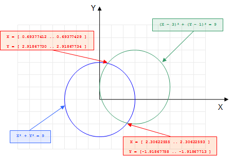
Fig. 3 Finding the intersection of two circles problem
In the previous chapter, we restricted ourselves to the cases where the variables take their value in a finite set of integer values. But in the two circles intersection problem, some of the decisions variables (the cartesian coordinates of the intersection(s) point(s)) are naturally continuous. One solution to model this problem with integer variables would be to scale the problem, ie: multiply by  all the coordinates to obtain only integers coordinates. This approach, even if it can work on some simple problems is very limitated:
First, it denaturates the problem and makes the modelisation less explicit.
Secondly, this approach would lead to huge variables domains and to very poor solving performances. This is due to the intrinsical nature of the filtering algorithms involved in the propagation of constraints between integer variables.
In order to tackle this kind of numerical problems, Artelys Kalis offers another type of variables: continuous variable that can take their value in an infinite set of values belonging to a closed interval of real numbers.
Adding continuous variables to the problem
Continuous variables are represented in Artelys Kalis by instances of the class KFloatVar. A key difference between KIntVar and KFloatVar is the domain representation of the variables. Unlike integer decision variables, continuous variables do not require a bounded domain and can take an infinite number of values. Before going further, we will review some key notions about numerical computations.
Numerical computations are based on the fundamental notion of floating point numbers. We note the set  as the set of real number augmented with the two infinite
values. And we define
as the set of real number augmented with the two infinite
values. And we define  , the set of floating points numbers as a finite part of
  containing
  and
and  . We note
  (respectively
  ) the successor (respectively predecessor) of a floating point number, with the additional convention that
  and
and  . We also define the following rounding operations:
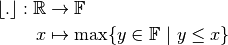
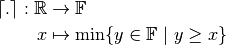
and for each real number  ,
, ![x=[\lfloor{x}\rfloor,\lceil{x}\rceil]](_images/math/27fdbf950d43e601b3f31ca995d3e17c316ae9b6.png) .
.
Coming back to Artelys Kalis, how can we represent continuous variables ? As seen above, using a finite set representation would lead to potential domains size of  elements (number of floating points numbers that nowadays typical computers can represent) which is prohibitive. The representation adopted by Artelys Kalis is an approximation of the variable by an interval
 ![[LB, UB]](_images/math/657498ce3cf94dbaf57542dc7230a2c53a553466.png) where
where  and
and  belong to the set of floating points numbers. An immediate consequence of this approximated representation is the fact that the solver can no more remove infeasible values in the interval
 ![]LB, UB[](_images/math/6f34d97c6bbfd7da27221cdb76b4cdd637cf3f3f.png) . Instead the solver ensures that all the solutions are contained in the hyper box defined by the union of the interval representation of the numerical variables. The figure Fig. 4 shows the hyperbox containing all the solutions of the intersection problem:
. Instead the solver ensures that all the solutions are contained in the hyper box defined by the union of the interval representation of the numerical variables. The figure Fig. 4 shows the hyperbox containing all the solutions of the intersection problem:
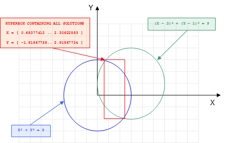
Fig. 4 Hyperbox containing all the solutions of the intersection problem
When do we consider that a continuous variable is instantiated? In the case of an integer valued variable, the answer is straightforward: when the domain of the variable is reduced to a singleton. But in the case of the continuous variable, the answer depends on user’s needs. One possibility would be to consider a continuous variable as instantiated as soon as its interval representation is reduced to an interval of type  where is a floating point number. However this approach would be computationally prohibitive. To allow a reasonable resolution time, a solution is to introduce a precision for each variable representing the domain size under which we can consider a continuous variable as instantiated. We can distinct two kind of precisions: absolute precision
  and relative precision:
 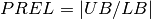 .
.
Fig. 5 Instantiation of a continuous variable
For instance, for a continuous variable  with a domain
 ![[10.0 .. 10.0001]](_images/math/fb78162c7337905ac8604ef7deac2034f94e324c.png) would be considered as instantiated if its absolute precision is less or equal to
would be considered as instantiated if its absolute precision is less or equal to  or if its relative precision is less or equal to
  .
.
Now that we know how continuous variables are represented in Artelys Kalis, let’s see how we can create such variables. We will use the different constructors of KFloatVar for this task.
The simplest constructor uses two parameters:
The first parameter
pcorresponds to the problem to which the variable belongs.The second is the name of the continuous variable that will be created.
KFloatVar * x = new KFloatVar(p, "x");
KFloatVar * y = new KFloatVar(p, "y");
x = KFloatVar(p, "x")
y = KFloatVar(p, "y")
KFloatVar x = new KFloatVar(p,"x");
KFloatVar y = new KFloatVar(p,"y");
The previous example creates two continuous variables named x and y with an initial infinite domain ![[-\infty \ldots +\infty]](_images/math/1dfdea960be78b42a39794eb45173190fa6f24a0.png) and a default precision.
and a default precision.
Another constructor uses six parameters:
The first parameter corresponds to the problem to which the variable belongs.
The second is the name of the continuous variable that will be created.
The third corresponds to the lower bound of the interval representing the domain of the variable.
The fourth corresponds to the upper bound of the interval representing the domain of the variable.
The fifth is a Boolean that indicates the kind of precision for this variable (
KFloatVar::PABSOLUTEfor absolute precision andKFloatVar.PRELATIVEfor relative precision).The last argument corresponds to the quantification of the precision.
KFloatVar * x = new KFloatVar(p,"x",-3.2,1.5,KFloatVar::PABSOLUTE,1e-5);
KFloatVar * y = new KFloatVar(p,"y",1, KFloatVar::PINFINITY,KFloatVar::PRELATIVE , 1e-6);
x = KFloatVar(p, "x", -3.2, 1.5, KFloatVar.PABSOLUTE, 1e-5)
y = KFloatVar(p, "y", 1, float("inf"), KFloatVar.PRELATIVE, 1e-6)
KFloatVar x = new KFloatVar(p,"x",-3.2,1.5, KFloatVar.PABSOLUTE > 0,1e-5);
KFloatVar y = new KFloatVar(p,"y",1, Double.POSITIVE_INFINITY,KFloatVar.PABSOLUTE > 0, 1e-6);
In this code, one continuous variable with an initial domain ![[-3.2 .. 1.5]](_images/math/3d066fc3980d1d318c1b60442b166610280d6086.png) and an absolute precision of
and an absolute precision of  , and a second variable y with an initial domain
 ![[1...+\infty]](_images/math/b1fd2fb7250d308b9ae9235336a1eada05ccb08b.png) and a relative precision of
and a relative precision of  would be created.
Note that the KFloatVar class derives directly from the KNumVar class, exactly like KIntVar. The KNumVar class is an abstract super class of all the numerical variables in Artelys Kalis. As an abstract class, KNumVar cannot be directly instantiated but can be used to gather independently all instances of the derived classes:
KNumVar * var;
var = new KFloatVar(p, "Continuous variable");
var = new KIntVar(p, "Finite domain variable", 0, 1);
def addOne(x : KNumVar):
    return x + 1
addOne(KFloatVar(p, "Continuous variable"))
addOne(KIntVar(p, "Finite domain variable", 0, 1))
KNumVar var = new KNumVar();
var = new KFloatVar(p, "Continuous variable");
var = new KIntVar(p, "Finite domain variable", 0, 1);
KFloatVar and KIntVar objects can be gathered to KNumVarArray: this class represents ordered sets of numeric variables and is the direct extension of the class KIntVarArray to numerical variables:
KNumVarArray myArray;
myArray.add(new KFloatVar(p, "Continuous variable"));
myArray.add(new KIntVar(p, "Finite domain variable", 0, 1));
myArray = KNumVarArray()
myArray += KFloatVar(p, "Continuous variable")
myArray += KIntVar(p, "Finite domain variable", 0, 1)
KNumVarArray myArray = new K;
myArray.add(new KFloatVar(p, "Continuous variable"));
myArray.add(new KIntVar(p, "Finite domain variable", 0, 1));
Posting constraints to the problem
The first constraint concerns the fact that the intersection points belong to the first circle, thus it must satisfy the equation  . Such a constraint is not a basic constraint in Artelys Kalis so we will need to decompose it into several basics constraints linked by additional intermediary variables that are not directly related to the problem.
For example, Artelys Kalis handles the following basic constraints:
Constraint |
Implementation class |
|---|---|
|
|
|
|
|
|
|
|


We can rewrite the constraint in:
square_radius = radius2
square_x = x2
square_y = y2
square_radius = square_x + square_y
Translated into Artelys Kalis one obtains the following code:
p.post(new KNumXEqualsYSquared(square_radius, radius));
p.post(new KNumXEqualsYSquared(square_x, x));
p.post(new KNumXEqualsYSquared(square_y, y));
p.post(new KNumEqualXYZ(square_radius, square_x, square_y));
p.post(KNumXEqualsYSquared(square_radius, radius))
p.post(KNumXEqualsYSquared(square_x, x))
p.post(KNumXEqualsYSquared(square_y, y))
p.post(KNumEqualXYZ(square_radius, square_x, square_y))
p.post(new KNumXEqualsYSquared(square_radius, radius));
p.post(new KNumXEqualsYSquared(square_x, x));
p.post(new KNumXEqualsYSquared(square_y, y));
p.post(new KNumEqualXYZ(square_radius, square_x, square_y));
Similarly, the constraint  can be decomposed in:
translated_x = x – 3
translated_y = y – 1
square_translated_x = translated_x2
square_translated_y = translated_y2
square_radius = square_translated_x + square_translated_y
Thus resulting into the following code:
// translation
KFloatVar translatedX(p, "x-3");
KFloatVar translatedY(p, "y-1");
p.post(new KNumEqualXYc(translatedX, x, -3));
p.post(new KNumEqualXYc(translatedY, y, -1));

// distance to the second circle center
KFloatVar squareTranslatedX(p, "(x-3)^2");
KFloatVar squareTranslatedY(p, "(y-1)^2");
p.post(new KNumXEqualsYSquared(squareTranslatedX, translatedX));
p.post(new KNumXEqualsYSquared(squareTranslatedY, translatedY));
p.post(new KNumEqualXYZ(squareRadius, squareTranslatedX, squareTranslatedY));
# translation
translated_x = KFloatVar(p, "x-3")
translated_y = KFloatVar(p, "y-1")
p.post(KNumEqualXYc(translated_x, x, -3))
p.post(KNumEqualXYc(translated_y, y, -1))

# distance to the second circle center
square_translated_x = KFloatVar(p, "(x-3)^2")
square_translated_y = KFloatVar(p, "(y-1)^2")
p.post(KNumXEqualsYSquared(square_translated_x, translated_x))
p.post(KNumXEqualsYSquared(square_translated_y, translated_y))
p.post(KNumEqualXYZ(square_radius, square_translated_x, square_translated_y))
// translation
KFloatVar translated_x = new KFloatVar(p, "x-3");
KFloatVar translated_y = new KFloatVar(p, "y-1");
p.post(new KNumEqualXYc(translated_x, x, -3));
p.post(new KNumEqualXYc(translated_y, y, -1));

// distance to the second circle center
KFloatVar square_translated_x = new KFloatVar(p, "(x-3)^2");
KFloatVar square_translated_y = new KFloatVar(p, "(y-1)^2");
p.post(new KNumXEqualsYSquared (square_translated_x,translated_x));
p.post(new KNumXEqualsYSquared (square_translated_y,translated_y));
p.post(new KNumEqualXYZ(square_radius, square_translated_x, square_translated_y));
Solving the problem
The problem is solved in the same manner as in the Personnal planning example. We simply create an instance of the KSolver object on the problem, and use the findAllSolutionsMethod() to find all the solutions of the problem:
KSolver solver(p);

int nbSol = solver.findAllSolutions();
solver = KSolver(p)
nbSol = solver.findAllSolutions()
KSolver solver = new KSolver(p);
Then we explore the solutions with the KProblem::getSolution() method of the class KProblem:
for (int i = 0; i < nbSol; i++)
{
    printf("-----------------------------------\n");
    printf("** Solution number %i\n" , i);
    printf("-----------------------------------\n");
    KSolution * sol = &p.getSolution(i);
    sol->print();
}
for i in range(nb_sol):
    print("-----------------------------------")
    print("** Solution number %d" % i)
    print("-----------------------------------")
    sol = p.getSolution(i)
    sol.display()
int nbSol = solver.findAllSolutions();
for (int i = 0; i < nbSol; i++)
{
    System.out.println("-----------------------------------");
    System.out.println("** Solution number " + i);
    System.out.println("-----------------------------------");
    p.getSolution(i).print();
}
Example summary
Below is the complete source code for solving the Two circles intersection problem.
KFloatVar::setDefaultPrecisionParameters(KFloatVar::PABSOLUTE, 1e-6);

KFloatVar x(p, "x");
KFloatVar y(p, "y");

KFloatVar::setDefaultPrecisionParameters(KFloatVar::PABSOLUTE, KFloatVar::PINFINITY);

KIntVar radius(p, "radius", 0, 5);
KIntVar square_radius(p, "squared radius",0,25);

p.post(KNumXEqualsYSquared(square_radius, radius));
// distance to the center of the first circle
KFloatVar square_x(p, "x^2");
KFloatVar square_y(p, "y^2");
p.post(KNumXEqualsYSquared(square_x, x));
p.post(KNumXEqualsYSquared(square_y, y));
//p.post(new KNumXEqualsYArithPowC(square_x, x, 2));
//p.post(new KNumXEqualsYArithPowC(square_y, y, 2));
//p.post (new KNumXEqualsYTimesZ (square_x, x, x));
//p.post (new KNumXEqualsYTimesZ (square_y, y, y));

p.post(KNumEqualXYZ(square_radius, square_x, square_y));

// translation
KFloatVar translated_x(p, "x-3");
KFloatVar translated_y(p, "y-1");
p.post(KNumEqualXYc(translated_x, x, -3));
p.post(KNumEqualXYc(translated_y, y, -1));

// distance to the second circle center
KFloatVar square_translated_x(p, "(x-3)^2");
KFloatVar square_translated_y(p, "(y-1)^2");
p.post (KNumXEqualsYSquared (square_translated_x,translated_x));
p.post (KNumXEqualsYSquared (square_translated_y,translated_y));
//p.post (new KNumXEqualsYArithPowC(square_translated_y,translated_y,2));
//p.post(new KNumXEqualsYTimesZ(square_translated_x, translated_x, translated_x));
//p.post(new KNumXEqualsYTimesZ(square_translated_y, translated_y, translated_y));
p.post(KNumEqualXYZ(square_radius, square_translated_x, square_translated_y));

p.propagate();
printf("\n-----------------------------------\n");
printf("-- After the initial propagation --\n");
printf("-----------------------------------\n");
p.print();

KSolver solver(p);

int nbSol = solver.findAllSolutions();
for (int i = 0; i < nbSol; i++)
{
    printf("-----------------------------------\n");
    printf("** Solution number %i\n" , i);
    printf("-----------------------------------\n");
    p.getSolution(i).print();
}
KFloatVar.setDefaultPrecisionParameters(KFloatVar.PABSOLUTE, 1e-6)

x = KFloatVar(p, "x")
y = KFloatVar(p, "y")

KFloatVar.setDefaultPrecisionParameters(KFloatVar.PABSOLUTE, float("inf"))

radius = KIntVar(p, "radius", 0, 5)
square_radius = KIntVar(p, "squared radius",0,25)

p.post(KNumXEqualsYSquared(square_radius, radius))
# distance to the center of the first circle
square_x = KFloatVar(p, "x^2")
square_y = KFloatVar(p, "y^2")
p.post(KNumXEqualsYSquared(square_x, x))
p.post(KNumXEqualsYSquared(square_y, y))
#p.post(KNumXEqualsYArithPowC(square_x, x, 2))
#p.post(KNumXEqualsYArithPowC(square_y, y, 2))
#p.post(KNumXEqualsYTimesZ (square_x, x, x))
#p.post(KNumXEqualsYTimesZ (square_y, y, y))

p.post(KNumEqualXYZ(square_radius, square_x, square_y))

# translation
translated_x = KFloatVar(p, "x-3")
translated_y = KFloatVar(p, "y-1")
p.post(KNumEqualXYc(translated_x, x, -3))
p.post(KNumEqualXYc(translated_y, y, -1))

# distance to the second circle center
squaretranslated_x = KFloatVar(p, "(x-3)^2")
squaretranslated_y = KFloatVar(p, "(y-1)^2")
p.post(KNumXEqualsYSquared(squaretranslated_x, translated_x))
p.post(KNumXEqualsYSquared(squaretranslated_y, translated_y))
#p.post(KNumXEqualsYArithPowC(squaretranslated_y, translated_y, 2))
#p.post(KNumXEqualsYTimesZ(squaretranslated_x, translated_x, translated_x))
#p.post(KNumXEqualsYTimesZ(squaretranslated_y, translated_y, translated_y))
p.post(KNumEqualXYZ(square_radius, squaretranslated_x, squaretranslated_y))

p.propagate()
print("-----------------------------------")
print("-- After the initial propagation --")
print("-----------------------------------")
p.display()

solver = KSolver(p)

nbSol = solver.findAllSolutions()
for i in range(nbSol):
    print("-----------------------------------")
    print("** Solution number %d" % i)
    print("-----------------------------------")
    sol = p.getSolution(i)
    sol.display()
KSession s = new KSession();

KProblem p = new KProblem(s, "TwoCirclesIntersection");

KFloatVar.setDefaultPrecisionParameters(KFloatVar.PABSOLUTE > 0, 1e-6);

KFloatVar x = new KFloatVar(p, "x");
KFloatVar y = new KFloatVar(p, "y");

KFloatVar.setDefaultPrecisionParameters(KFloatVar.PABSOLUTE > 0, Double.POSITIVE_INFINITY);

KIntVar radius = new KIntVar(p, "radius", 0, 5);
KIntVar square_radius = new KIntVar(p, "squared radius",0,25);

p.post(new KNumXEqualsYSquared(square_radius, radius));
// distance to the center of the first circle
KFloatVar square_x = new KFloatVar(p, "x^2");
KFloatVar square_y = new KFloatVar(p, "y^2");
p.post(new KNumXEqualsYSquared(square_x, x));
p.post(new KNumXEqualsYSquared(square_y, y));
//p.post(new KNumXEqualsYArithPowC(square_x, x, 2));
//p.post(new KNumXEqualsYArithPowC(square_y, y, 2));
//p.post (new KNumXEqualsYTimesZ (square_x, x, x));
//p.post (new KNumXEqualsYTimesZ (square_y, y, y));

p.post(new KNumEqualXYZ(square_radius, square_x, square_y));

// translation
KFloatVar translated_x = new KFloatVar(p, "x-3");
KFloatVar translated_y = new KFloatVar(p, "y-1");
p.post(new KNumEqualXYc(translated_x, x, -3));
p.post(new KNumEqualXYc(translated_y, y, -1));

// distance to the second circle center
KFloatVar square_translated_x = new KFloatVar(p, "(x-3)^2");
KFloatVar square_translated_y = new KFloatVar(p, "(y-1)^2");
p.post(new KNumXEqualsYSquared (square_translated_x,translated_x));
p.post(new KNumXEqualsYSquared (square_translated_y,translated_y));
//p.post (new KNumXEqualsYArithPowC(square_translated_y,translated_y,2));
//p.post(new KNumXEqualsYTimesZ(square_translated_x, translated_x, translated_x));
//p.post(new KNumXEqualsYTimesZ(square_translated_y, translated_y, translated_y));
p.post(new KNumEqualXYZ(square_radius, square_translated_x, square_translated_y));

p.propagate();
System.out.println("\n-----------------------------------");
System.out.println("-- After the initial propagation --");
System.out.println("-----------------------------------");
p.print();

KSolver solver = new KSolver(p);

int nbSol = solver.findAllSolutions();
for (int i = 0; i < nbSol; i++)
{
    System.out.println("-----------------------------------");
    System.out.println("** Solution number " + i);
    System.out.println("-----------------------------------");
    p.getSolution(i).print();
}