Termination criteria
This section describes the stopping tests used by Knitro to declare (local) optimality, and the corresponding user options that can be used to enforce more or less stringent tolerances in these tests.
Continuous problems
The first-order conditions for identifying a locally optimal solution are:
![\begin{gather}
\nabla_x {\cal L}(x,\lambda) =
\nabla f(x) + \sum_{i=0}^{m-1}\lambda^c_i\nabla c_i(x) + \lambda^b =0 \tag{1} \\
\lambda^c_i \min[(c_i(x)-c^L_i),(c^U_i-c_i(x))] = 0, \quad i=0,\ldots,m-1 \tag{2} \\
\lambda^b_j \min[(x_j-b^L_j),(b^U_j-x_j)] = 0, \quad j=0,\ldots,n-1 \tag{2b} \\
c^L_i \; \le \; c_i(x) \le c^U_i, \quad i=0,\ldots,m-1 \tag{3} \\
b^L_j \; \le \; x_j \le b^U_j, \quad j=0,\ldots,n-1 \tag{3b} \\
\lambda^c_i \ge 0, \quad i \in {\cal I}, \; c^L_i \mbox{ infinite }, \; c^U_i \mbox{ finite } \tag{4} \\
\lambda^c_i \le 0, \quad i \in {\cal I}, \; c^U_i \mbox{ infinite }, \; c^L_i \mbox{ finite } \tag{4b} \\
\lambda^b_j \ge 0, \quad j \in {\cal B}, \; b^L_j \mbox{ infinite }, \; b^U_j \mbox{ finite } \tag{5} \\
\lambda^b_j \le 0, \quad j \in {\cal B}, \; b^U_j \mbox{ infinite }, \; b^L_j \mbox{ finite }. \tag{5b}
\end{gather}](../_images/math/6ae6f74e46d571d88cbd942c9d88896bbfe12a40.png)
Here  and
and  represent the sets of indices corresponding
to the general inequality constraints and (non-fixed) variable bound constraints respectively.
In the conditions above,
represent the sets of indices corresponding
to the general inequality constraints and (non-fixed) variable bound constraints respectively.
In the conditions above,  is the Lagrange multiplier
corresponding to constraint
is the Lagrange multiplier
corresponding to constraint  , and
, and  is the Lagrange multiplier corresponding to the simple bounds on the
variable
is the Lagrange multiplier corresponding to the simple bounds on the
variable  . There is exactly one Lagrange multiplier
for each constraint and variable. The Lagrange multiplier may be
restricted to take on a particular sign depending on whether the
corresponding constraint (or variable) is upper bounded or lower
bounded, as indicated by (4)-(5). If the constraint (or variable)
has both a finite lower and upper bound, then the appropriate sign
of the multiplier depends on which bound (if either) is binding
(active) at the solution.
. There is exactly one Lagrange multiplier
for each constraint and variable. The Lagrange multiplier may be
restricted to take on a particular sign depending on whether the
corresponding constraint (or variable) is upper bounded or lower
bounded, as indicated by (4)-(5). If the constraint (or variable)
has both a finite lower and upper bound, then the appropriate sign
of the multiplier depends on which bound (if either) is binding
(active) at the solution.
In Knitro we define the feasibility error FeasErr at a point
 to be the maximum violation of the constraints
(3), (3b), i.e.,
to be the maximum violation of the constraints
(3), (3b), i.e.,

while the optimality error (OptErr) is defined as the maximum violation of the first three conditions (1)-(2b), with a small modification to conditions (2) and (2b). In these complementarity conditions, we really only need that either the multiplier or the corresponding constraint is 0, so we change the terms on the left side of these conditions to:
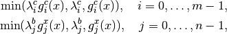
where
![g^c_i(x) = \min[(c_i(x)-c^L_i),(c^U_i-c_i(x))], \\
g^x_j(x) = \min[(x_j-b^L_j),(b^U_j-x_j)],](../_images/math/04e795d476ff52c779608e4d04b869cd0344de3f.png)
to protect against numerical problems that may occur when the Lagrange multipliers become very large. The remaining conditions on the sign of the multipliers (4)-(5b) are enforced explicitly throughout the optimization.
In order to take into account problem scaling in the termination test, the following scaling factors are defined
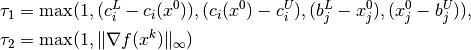
where  represents the initial point.
For unconstrained problems, the scaling factor  is not
effective since
is not
effective since 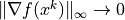 as a solution
is approached.
Therefore, for unconstrained problems only, the following scaling is
used in the termination test
as a solution
is approached.
Therefore, for unconstrained problems only, the following scaling is
used in the termination test

in place of .
Knitro stops and declares locally optimal solution found if the following stopping conditions are satisfied:

where feastol, opttol, feastol_abs,
and opttol_abs are constants defined by user options.
This stopping test is designed to give the user much flexibility in
deciding when the solution returned by Knitro is accurate enough.
By default, Knitro uses a scaled stopping test, while also enforcing
that some minimum absolute tolerances for feasibility and optimality
are satisfied.
One can use a purely absolute stopping test by setting
feastol_abs <= feastol and
opttol_abs <= opttol.
Finite-difference gradients
Note that the optimality condition (1) depends on gradient values of the
nonlinear objective and constraint functions.
When using finite-difference gradients (e.g. gradopt > 1), there
will typically be small errors in the computed gradients that will
limit the precision in the solution (and the ability to satisfy the optimality conditions).
By default, Knitro will try to estimate these finite-difference gradient errors
and terminate when it seems that no more accuracy in the solution is possible.
The solution will be treated as optimal as long as it is feasible and the
optimality conditions are satisfied either by the optimality tolerances used in (stop2)
or the error estimates.
This special termination can be disabled by setting findiff_terminate = 0 (none).
Scaling
Note that the optimality conditions (stop2) apply to the problem
being solved internally by Knitro. If the user option scale is enabled to
perform some scaling of the problem,
then the problem objective and constraint functions as well as the variables
may first be scaled
before the problem is sent to Knitro for the optimization. In this case,
the optimality conditions apply to the scaled form of the problem. If the accuracy
achieved by Knitro with the default settings is not satisfactory, the user
may either decrease the tolerances described above, or try setting scale = no.
Note that scaling the variables or constraints
in the problem via the scale user option and scaling/modifying the
stopping
tolerances are two different things. You should use scale to try to
make the variables/constraints in your model all have roughly the same
magnitude (e.g. close to 1) so that the Knitro algorithms work better.
Separately you should use the Knitro stopping tolerances to specify how much accuracy
you require in the solution.
Complementarity constraints
The feasibility error for a complementarity constraint is
measured as  where
where  and
and  are non-negative variables
that are complementary to each other. The tolerances defined by (stop1) are used
for determining feasibility of complementarity constraints.
are non-negative variables
that are complementary to each other. The tolerances defined by (stop1) are used
for determining feasibility of complementarity constraints.
Constraint specific feasibility tolerances
By default Knitro applies the same feasibility stopping tolerances
feastol / feastol_abs to all constraints. However,
it is possible for you to define an (absolute) feasibility tolerance
for each individual constraint in case you want to customize how feasible
the solution needs to be with respect to each individual constraint.
This can be done using the callable library API functions
KN_set_con_feastols(), KN_set_var_feastols(),
and KN_set_compcon_feastols(), which allows you to define custom
tolerances for the general constraints, the variable bounds and
any complementarity constraints.
Please see section
Callable library API reference for more details on these API functions. When using the
AMPL modeling language, the same feature can be used by defining the AMPL
input suffixes cfeastol and xfeastol for each constraint or variable
in your model.
Discrete or mixed integer problems
Algorithms for solving optimization problems where one or more of the variables are restricted to take on only discrete values, proceed by solving a sequence of continuous relaxations, where the discrete variables are relaxed such that they can take on any continuous value.
The best global solution of these relaxed problems,  ,
provides a lower bound on the optimal objective value for the original
problem (upper bound if maximizing).
If a feasible point is found for the relaxed problem that satisfies
the discrete restrictions on the variables, then this provides an upper bound on the
optimal objective value of the original problem (lower bound if maximizing).
We will refer to these feasible points as incumbent points and denote
the objective value at an incumbent point by
,
provides a lower bound on the optimal objective value for the original
problem (upper bound if maximizing).
If a feasible point is found for the relaxed problem that satisfies
the discrete restrictions on the variables, then this provides an upper bound on the
optimal objective value of the original problem (lower bound if maximizing).
We will refer to these feasible points as incumbent points and denote
the objective value at an incumbent point by  .
Assuming all the continuous subproblems have been solved to global
optimality (if the problem is convex, all local solutions are global solutions),
an optimal solution of the original problem is verified when the lower
bound and upper bound are equal.
.
Assuming all the continuous subproblems have been solved to global
optimality (if the problem is convex, all local solutions are global solutions),
an optimal solution of the original problem is verified when the lower
bound and upper bound are equal.
Knitro declares optimality for a discrete problem when the gap between the best
(i.e., largest) lower bound  and the best (i.e., smallest)
upper bound
and the best (i.e., smallest)
upper bound  is less than a threshold determined by the user options,
mip_opt_gap_abs and mip_opt_gap_rel.
Specifically, Knitro declares optimality when either

or

where mip_opt_gap_abs and mip_opt_gap_rel are typically
small positive numbers.
Since these termination conditions assume that the continuous subproblems
are solved to
global optimality and Knitro only finds local solutions of non-convex, continuous
optimization problems, they are only reliable when solving convex,
mixed integer problems.
The optimality gap 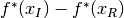 should be non-negative although
it may become slightly negative from roundoff error, or if the continuous subproblems
are not solved to sufficient accuracy.
If the optimality gap becomes largely negative, this may be an indication
that the model is non-convex, in which case Knitro may not converge to the optimal
solution, and will be unable to verify optimality (even if it claims otherwise).
should be non-negative although
it may become slightly negative from roundoff error, or if the continuous subproblems
are not solved to sufficient accuracy.
If the optimality gap becomes largely negative, this may be an indication
that the model is non-convex, in which case Knitro may not converge to the optimal
solution, and will be unable to verify optimality (even if it claims otherwise).