Scheduling

This chapter shows how to

• define and setup the modeling objects KTask and KResource,

• formulate and solve scheduling problems using these objects,

• access information from the modeling objects.

Tasks, resources and schedules

Scheduling and planning problems are concerned with determining a plan for the execution of a given set of tasks. The objective may be to generate a feasible schedule that satisfies the given constraints (such as sequence of tasks or limited resource availability) or to optimize a given criterion such as the makespan of the schedule. Artelys-Kalis defines several aggregate modeling objects to simplify the formulation of standard scheduling problems like tasks,resources and schedule objects. When working with these scheduling objects it is often sufficient to state the objects and their properties, such as task duration or resource use; the necessary constraint relations are set up automatically by Artelys-Kalis (referred to as implicit constraints). Before going further into the exploration of Artelys-Kalis scheduling capabilities, let’s first recall some basic concepts about scheduling problems and their modelisation that will be intensively used within this chapter.

Tasks

Tasks (processing operations, activities) are represented by the class KTask. This object contains three variables:

• a start variable representing the starting time of the task

• an end variable representing the ending time of the task

• a duration variable representing the duration of the task

These three structural variables are linked by Artelys-Kalis with the following constraint: .

The starting time variable represents two specific parameters of the task: * the Earliest Starting Time (EST represented by the start variable lower bound) * and its Latest Starting Time (LST represented by the start variable upper bound).

The end variable represents two specific parameters of the task: * the Earliest Completion Time (ECT represented by the end variable lower bound) * and its Latest Completion Time (LCT represented by the end variable upper bound).

The duration variable represents two specific parameters of the task: * the minimum task duration (Dmin represented by the duration variable lower bound) * the maximum task duration (Dmax represented by the duration variable upper bound).

The picture below illustrates this:

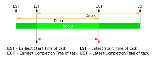
Fig. 8 Illustration of EST, ECT, LST and LCT paramters

Resources

Resources (machines, raw material etc.) can be of two different types:

• Disjunctive when the resource can process only one task at a time (represented by the class KunaryResource).

• Cumulative when the resource can process several tasks at the same time (represented by the class KdiscreteResource).

Traditional examples of disjunctive resources are Jobshop problems, cumulative resources are heavily used for the Resource-Constrained Project Scheduling Problem (RCPSP). Note that a disjunctive resource is semantically equivalent to a cumulative resource with maximal capacity one and unit resource usage for each task using this resource but this equivalence does not hold in terms of constraint propagation.

The following schema shows an example with three tasks A,B and C executing on a disjunctive resource and on a cumulative resource with resource usage 3 for task A, 1 for task B and 1 for task C:

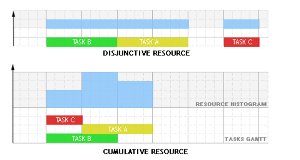
Fig. 9 Disjunctive and cumulative resources

Tasks may require, provide, consume and produce resources:

• A task requires a resource if some amount of the resource capacity must be made available for the execution of the activity. The capacity is renewable which means that the required capacity is available after the end of the task.

• A task provides a resource if some amount of the resource capacity is made available through the execution of the task. The capacity is renewable which means that the provided capacity is available only during the execution of the task.

• A task consumes a resource if some amount of the resource capacity must be made available for the execution of the task and the capacity is non-renewable which means that the consumed capacity if no longer available at the end of the task.

• A task produces a resource if some amount of the resource capacity is made available at the end of the task and the capacity is non-renewable which means that the produced capacity is definitively available after the task completion.

Schedule

Tasks and resources are gathered into a schedule. The method KSchedule::optimize() allows to optimize a schedule relatively to any objective variable (defined via the method KSchedule::setObjective() and implements advanced scheduling techniques specialized in makespan minimization. The creation of the schedule makespan can be automated by calling the KSchedule::getMakespan() method that ensures automatically its computation.

Artelys-Kalis Built-In Scheduler

In the following sections we show a number of examples using this mechanism:

• The simplest case of a scheduling problem involves only tasks and precedence constraints between tasks (project scheduling problem in Section 11.2).

• Tasks may be mutually exclusive, e.g. because they use the same unitary resource (disjunctive scheduling / sequencing problem in Section 11.3).

• Resources may be usable by several tasks at a time, up to a given capacity limit (cumulative resources, see Section 11.4).

• A different classification of resources is the distinction between renewable and nonrenewable resources (see Section 11.5).

• Many extensions of the standard problems are possible, such as sequence-dependent setup time (see Section 11.6).

If the enumeration is started with the methods KSchedule::schedule() the solver will employ specialized search strategies suitable for the corresponding (scheduling) problem type. However, it is also possible to employ parameterized search strategies or to define user search strategies for scheduling objects in this case the standard optimization functions KSolver::minimize() or KSolver::maximize() need to be used (see Section 11.7).

The properties of scheduling objects (such as start time or duration of tasks) can be accessed and employed, for instance, in the definition of constraints, thus giving the user the possibility to extend the predefined standard problems with other types of constraints. For even greater flexibility Artelys-Kalis also enables the user to formulate his scheduling problems without the aggregate modeling objects, using dedicated global constraints on decision variables of type KIntVar. Most examples in this chapter are therefore given with two different implementations, one using the scheduling objects and another without these objects.

Precedences

Probably the most basic type of a scheduling problem is to plan a set of tasks that are linked by precedence constraints. The problem described in this section is taken from Section 7.1 Construction of a stadium of the book Applications of optimization with Xpress-MP.

A construction company has been awarded a contract to construct a stadium and wishes to complete it within the shortest possible time. Figure Fig. 10 lists the major tasks and their durations in weeks. Some tasks can only start after the completion of certain other tasks, equally indicated in the table.

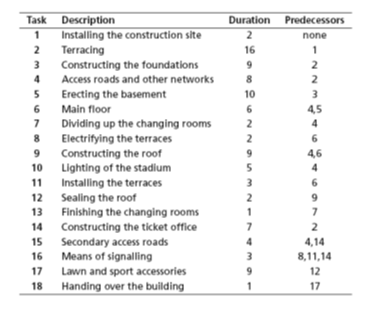
Fig. 10 Data for stadium construction

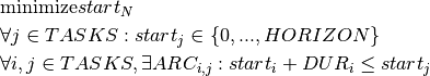
Model formulation

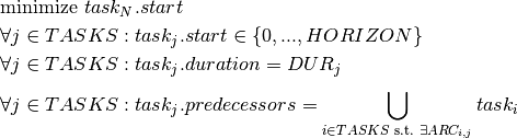
This problem is a classical project scheduling problem. We add a fictitious task with 0 duration that corresponds to the end of the project. We thus consider the set of tasks where is the fictitious end task. Every construction task () is represented by a KTask object with variable start time and a duration fixed to the given value . The precedences between tasks are represented by a precedence graph with arcs () symbolizing that task precedes task . The objective is to minimize the completion time of the project, that is the start time of the last, fictitious task . We thus obtain the following model where an upper bound on the start times is given by the sum of all task durations:

Implementation

The following model shows the implementation of this problem with Artelys-Kalis. Since there are no side-constraints, the earliest possible completion time of the schedule is the earliest start of the fictitious task . To trigger the propagation of task-related constraints we simply call the method KProblem::propagate() as usual. At this point, constraining the start of the fictitious end task to its lower bound reduces all task start times to their feasible intervals through the effect of constraint propagation. The start times of tasks on the critical path are fixed to a single value. The call to KSchedule::optimize() serves for instantiating all variables to their lower bounds.

C++PythonJava

// Number of tasks
int NTASKS = 19;
// Duration of tasks
int  DUR[] =  {2 ,16 , 9 , 8, 10,  6 , 2 , 2 , 9 , 5 , 3 , 2 , 1 , 7 , 4 , 3 , 9 , 1 , 0};
// Time horizon
int HORIZON;
// Tasks to be planned
KTaskArray task;
// best upper bound
int bestend;
// index variable
int indexTask;

// computing maximal time horizon;
HORIZON = 0;
for (indexTask = 0;indexTask < NTASKS; indexTask++) {
    HORIZON += DUR[indexTask];
}

// Creation of the problem in this session
KProblem problem(session,"B-1 Stadium construction");
// Creation of the schedule object with time horizon (0..HORIZON)
KSchedule schedule(problem,"B-1 Stadium construction schedule",0,HORIZON);

char name[80];
// building each task with fixed duration
for (indexTask = 0;indexTask < NTASKS; indexTask++) {
      sprintf(name,"T%i",indexTask);
    task += * (new KTask(schedule,name,DUR[indexTask]) ) ;
}

// setting the predecessors of each task
task[1].startsAfter(task[0]);
task[2].startsAfter(task[1]);
task[3].startsAfter(task[1]);
task[13].startsAfter(task[1]);
task[4].startsAfter(task[2]);
task[5].startsAfter(task[3]);
task[6].startsAfter(task[3]);
task[8].startsAfter(task[3]);
task[9].startsAfter(task[3]);
task[14].startsAfter(task[3]);
task[5].startsAfter(task[4]);
task[7].startsAfter(task[5]);
task[8].startsAfter(task[5]);
task[10].startsAfter(task[5]);
task[12].startsAfter(task[6]);
task[15].startsAfter(task[7]);
task[11].startsAfter(task[8]);
task[18].startsAfter(task[9]);
task[15].startsAfter(task[10]);
task[16].startsAfter(task[11]);
task[18].startsAfter(task[12]);
task[14].startsAfter(task[13]);
task[15].startsAfter(task[13]);
task[18].startsAfter(task[14]);
task[18].startsAfter(task[15]);
task[17].startsAfter(task[16]);
task[18].startsAfter(task[17]);

// propagating problem
if (problem.propagate()) {
    printf("Problem is infeasible\n");
    exit(1);
}
// Since there are no side-constraints, the earliest possible completion
// time is the earliest start of the fictitious task N
bestend = task[NTASKS-1].getStartDateVar()->getInf();
task[NTASKS-1].getStartDateVar()->setSup(bestend);
printf("Earliest possible completion time: %i\n", bestend);

// For tasks on the critical path the start/completion times have been fixed
// by setting the bound on the last task. For all other tasks the range of
// possible start/completion times gets displayed.
for (indexTask = 0;indexTask < NTASKS; indexTask++) {
    printf("%i:",indexTask);
    task[indexTask].getStartDateVar()->print();
    printf("\n");
}
// Complete enumeration: schedule every task at the earliest possible date
int result = schedule.optimize();

// solution printing
problem.getSolution().print();

Results

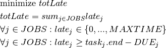
The earliest completion time of the stadium construction is 64 weeks. Here is a graphical representation of the solution:

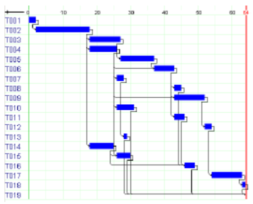
Fig. 11 Results of Stadium Construction example

Alternative formulation without scheduling objects

As for the previous formulation, we work with a set of tasks where is the fictitious end task. For every task we introduce a decision variable to denote its start time. With the duration of task , the precedence relation task i precedes task j is stated by the constraint :

We therefore obtain the following model for our project scheduling problem:

The corresponding model is printed in full below:

C++PythonJava

// Number of tasks
int NTASKS = 19;
// Duration of tasks
int  DUR[] =  {2 ,16 , 9 , 8, 10,  6 , 2 , 2 , 9 , 5 , 3 , 2 , 1 , 7 , 4 , 3 , 9 , 1 , 0};
// Time horizon
int HORIZON;
// Start dates of tasks to be planned
KIntVarArray starts;
// best upper bound
int bestend;
// index variable
int indexTask;

// computing maximal time horizon;
HORIZON = 0;
for (indexTask = 0;indexTask < NTASKS; indexTask++) {
    HORIZON += DUR[indexTask];
}

// Creation of the problem in this session
KProblem problem(session,"B-1 Stadium construction - Alt");

char name[80];
// building each tasks with fixed time horizon (0..HORIZON)
for (indexTask = 0;indexTask < NTASKS; indexTask++) {
      sprintf(name,"T%i",indexTask);
    starts += * (new KIntVar(problem,name,0,HORIZON) );
}

// setting the predecessors of each tasks
problem.post( starts[1]  >= starts[0] + DUR[0] );
problem.post( starts[2]  >= starts[1] + DUR[1] );
problem.post( starts[3]  >= starts[1] + DUR[1] );
problem.post( starts[13] >= starts[1] + DUR[1] );
problem.post( starts[4]  >= starts[2] + DUR[2] );
problem.post( starts[5]  >= starts[3] + DUR[3] );
problem.post( starts[6]  >= starts[3] + DUR[3] );
problem.post( starts[8]  >= starts[3] + DUR[3] );
problem.post( starts[9]  >= starts[3] + DUR[3] );
problem.post( starts[14] >= starts[3] + DUR[3] );
problem.post( starts[5]  >= starts[4] + DUR[4] );
problem.post( starts[7]  >= starts[5] + DUR[5] );
problem.post( starts[8]  >= starts[5] + DUR[5] );
problem.post( starts[10] >= starts[5] + DUR[5] );
problem.post( starts[12] >= starts[6] + DUR[6] );
problem.post( starts[15] >= starts[7] + DUR[7] );
problem.post( starts[11] >= starts[8] + DUR[8] );
problem.post( starts[18] >= starts[9] + DUR[9] );
problem.post( starts[15] >= starts[10] + DUR[10] );
problem.post( starts[16] >= starts[11] + DUR[11] );
problem.post( starts[18] >= starts[12] + DUR[12] );
problem.post( starts[14] >= starts[13] + DUR[13] );
problem.post( starts[15] >= starts[13] + DUR[13] );
problem.post( starts[18] >= starts[14] + DUR[14] );
problem.post( starts[18] >= starts[15] + DUR[15] );
problem.post( starts[17] >= starts[16] + DUR[16] );
problem.post( starts[18] >= starts[17] + DUR[17] );


// propagating problem
if (problem.propagate()) {
    printf("Problem is infeasible\n");
    exit(1);
}
// Since there are no side-constraints, the earliest possible completion
// time is the earliest start of the fictitious task N
bestend = starts[NTASKS-1].getInf();
starts[NTASKS-1].setSup(bestend);
printf("Earliest possible completion time: %i\n", bestend);

// For tasks on the critical path the start/completion times have been fixed
// by setting the bound on the last task. For all other tasks the range of
// possible start/completion times gets displayed.
for (indexTask = 0;indexTask < NTASKS; indexTask++) {
    printf("%i:",indexTask);
    starts[indexTask].print();
    printf("\n");
}
problem.setObjective(starts[18]);
problem.setSense(KProblem::Minimize);
KSolver solver(problem);
// Complete enumeration: schedule every task at the earliest possible date
int result = solver.optimize();

// solution printing
problem.getSolution().print();

Disjunctive scheduling: unary resources

The problem of sequencing jobs on a single machine described in Section 11.3 may be represented as a disjunctive scheduling problem using the KTask and KResource modeling objects. The reader is reminded that the problem is to schedule the processing of a set of non-preemptive tasks (or jobs) on a single machine. For every task its release date, duration, and due date are given. The problem is to be solved with three different objectives, mimizing the makespan, the average completion time, or the total tardiness.

Model formulation

The major part of the model formulation consists of the definition of the scheduling objects tasks and resources.

Every job () is represented by a task object , with a start time in 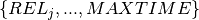(where is a sufficiently large value, such as the sum of all release dates and all durations, and the release date of job ) and the task duration fixed to the given processing time . All jobs use the same resource of unitary capacity. This means that at most one job may be processed at any one time, we thus implicitly state the disjunctions between the jobs. Another implicit constraint established by the task objects is the relation between the start, duration, and completion time of a job .

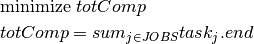
Objective 1: The first objective is to minimize the makespan (completion time of the schedule) or, equivalently, to minimize the completion time finish of the last job. The complete model is then given by the following (where is a sufficiently large value, such as the sum of all release dates and all durations):

Objective 2: The formulation of the second objective (minimizing the average processing time or, equivalently, minimizing the sum of the job completion times) remains unchanged from the first model we introduce an additional variable representing the sum of the completion times of all jobs.

Objective 3: To formulate the objective of minimizing the total tardiness, we introduce new variables to measure the amount of time that a job finishes after its due date. The value of these variables corresponds to the difference between the completion time of a job and its due date . If the job finishes before its due date, the value must be zero. The objective now is to minimize the sum of these tardiness variables:

The following implementation with Artelys-Kalis shows how to set up the necessary task and resource modeling objects. The resource is of the type KUnaryResource meaning that it processes at most one task at a time. For the tasks we use the constructor of KTask with the following signature:

C++PythonJava

KTask(KSchedule &s,const char * name,int duration,KResource & r);

The last parameter indicates that the task use the resource r with unitary ressource requirement. The latter exists in several versions for different combinations of arguments (task attributes) the reader is referred to the Artelys-Kalis Reference Manual for further detail.

C++PythonJava

// Number of tasks
int NTASKS = 7;

// Release date of tasks
int REL[] = { 2,  5,  4,  0,  0,  8,  9};
// Duration of tasks
int DUR[] = { 5,  6,  8,  4,  2,  4,  2};
// Due date of tasks
int DUE[] = {10, 21, 15, 10,  5, 15, 22};

// Time horizon
int MAXTIME;
// Tasks to be planned
KTaskArray task;
// best upper bound
int bestend;
// index variable
int indexTask;

// computing maximal time horizon;
int SUMDUR = 0;
for (indexTask = 0;indexTask < NTASKS; indexTask++) {
    SUMDUR += DUR[indexTask];
}
MAXTIME = 0;
for (indexTask = 0;indexTask < NTASKS; indexTask++) {
    if (REL[indexTask] + DUR[indexTask] > MAXTIME) {
        MAXTIME = REL[indexTask] + SUMDUR;
    }
}

// Creation of the problem in this session
KProblem problem(session,"B-4 Sequencing");
// Creation of the schedule object with time horizon (0..MAXTIME)
KSchedule schedule(problem,"B-4 Sequencing schedule",0,100);

// Resource (machine)
KUnaryResource cpresource(schedule,"machine");


char name[80];
// building each tasks with fixed duration
for (indexTask = 0;indexTask < NTASKS; indexTask++) {
    sprintf(name,"T%i",indexTask);
    task += * (new KTask(schedule,name,DUR[indexTask],cpresource) ) ;
    task[indexTask].getStartDateVar()->setInf(REL[indexTask]);
}

// propagating problem
if (problem.propagate()) {
    printf("Problem is infeasible\n");
    exit(1);
}


// **********************
// Objective 1: Makespan
// **********************

int result = schedule.optimize();
// solution printing
printf("Completion time: %i\n",problem.getSolution().getValue(*schedule.getMakeSpan()));
printf("Rel\t");
for (indexTask = 0;indexTask < NTASKS; indexTask++) {
printf("%i\t",REL[indexTask]);
}
printf("\nDur\t");
for (indexTask = 0;indexTask < NTASKS; indexTask++) {
    printf("%i\t",DUR[indexTask]);
}
printf("\nStart\t");
for (indexTask = 0;indexTask < NTASKS; indexTask++) {
    printf("%i\t",problem.getSolution().getValue(*task[indexTask].getStartDateVar()));
}
printf("\nEnd\t");
for (indexTask = 0;indexTask < NTASKS; indexTask++) {
    printf("%i\t",problem.getSolution().getValue(*task[indexTask].getEndDateVar()));
}
printf("\nDue\t");
for (indexTask = 0;indexTask < NTASKS; indexTask++) {
    printf("%i\t",DUE[indexTask]);
}
printf("\n");

// ***************************************
// Objective 2: Average completion time:
// ***************************************

KLinTerm totalCompletionTerm;
for (indexTask = 0;indexTask < NTASKS; indexTask++) {
    totalCompletionTerm = totalCompletionTerm + *task[indexTask].getEndDateVar();
}
KIntVar averageCompletion(problem,"average completion",0,1000);
problem.post(averageCompletion == totalCompletionTerm);


schedule.setObjective(averageCompletion);
result = schedule.optimize();
// solution printing
printf("Completion time: %i\n",problem.getSolution().getValue(*schedule.getMakeSpan()));
printf("average: %i\n",problem.getSolution().getValue(averageCompletion));
printf("Rel\t");
for (indexTask = 0;indexTask < NTASKS; indexTask++) {
    printf("%i\t",REL[indexTask]);
}
printf("\nDur\t");
for (indexTask = 0;indexTask < NTASKS; indexTask++) {
    printf("%i\t",DUR[indexTask]);
}
printf("\nStart\t");
for (indexTask = 0;indexTask < NTASKS; indexTask++) {
    printf("%i\t",problem.getSolution().getValue(*task[indexTask].getStartDateVar()));
}
printf("\nEnd\t");
for (indexTask = 0;indexTask < NTASKS; indexTask++) {
    printf("%i\t",problem.getSolution().getValue(*task[indexTask].getEndDateVar()));
}
printf("\nDue\t");
for (indexTask = 0;indexTask < NTASKS; indexTask++) {
    printf("%i\t",DUE[indexTask]);
}
printf("\n");

// *****************************
// Objective 3: total lateness:
// *****************************

KIntVarArray late;
KLinTerm totLatTerm;
// building each tasks with fixed time horizon (0..HORIZON)
for (indexTask = 0;indexTask < NTASKS; indexTask++) {
    sprintf(name,"late(%i)",indexTask);
    late += * (new KIntVar(problem,name,0,MAXTIME) );
    problem.post(late[indexTask] >= (*task[indexTask].getEndDateVar()) - DUE[indexTask]);
    totLatTerm = totLatTerm + late[indexTask];
}
KIntVar totLate(problem,"total lateness",0,1000);
problem.post(totLate == totLatTerm);

schedule.setObjective(totLate);
result = schedule.optimize();
// solution printing
printf("Completion time: %i\n",problem.getSolution().getValue(*schedule.getMakeSpan()));
printf("average: %i\n",problem.getSolution().getValue(averageCompletion));
printf("Tardiness: %i\n",problem.getSolution().getValue(totLate));
printf("Rel\t");
for (indexTask = 0;indexTask < NTASKS; indexTask++) {
    printf("%i\t",REL[indexTask]);
}
printf("\nDur\t");
for (indexTask = 0;indexTask < NTASKS; indexTask++) {
    printf("%i\t",DUR[indexTask]);
}
printf("\nStart\t");
for (indexTask = 0;indexTask < NTASKS; indexTask++) {
    printf("%i\t",problem.getSolution().getValue(*task[indexTask].getStartDateVar()));
}
printf("\nEnd\t");
for (indexTask = 0;indexTask < NTASKS; indexTask++) {
    printf("%i\t",problem.getSolution().getValue(*task[indexTask].getEndDateVar()));
}
printf("\nDue\t");
for (indexTask = 0;indexTask < NTASKS; indexTask++) {
    printf("%i\t",DUE[indexTask]);
}
printf("\nLate\t");
for (indexTask = 0;indexTask < NTASKS; indexTask++) {
    printf("%i\t",problem.getSolution().getValue(late[indexTask]));
}
printf("\n");

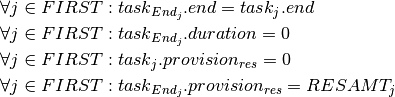
Results

This model produces similar results as those reported for the model versions in Section 11.3. Following figure shows the Gantt chart display of the solution. Above the Gantt chart we can see the resource usage display: the machine is used without interruption by the tasks, that is, even if we relaxed the constraints given by the release times and due dates it would not have been possible to generate a schedule terminating earlier.

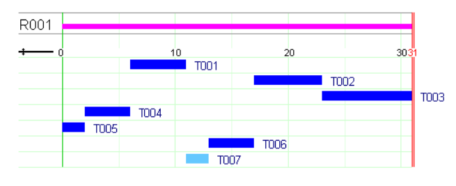
Fig. 12 Solution display

Cumulative scheduling: discrete resources

The problem described in this section is taken from Section 9.4 Backing up files of the book Applications of optimization with Xpress-MP.

Our task is to save sixteen files of the following sizes: 46kb, 55kb, 62kb, 87kb, 108kb, 114kb, 137kb, 164kb, 253kb, 364kb, 372kb, 388kb, 406kb, 432kb, 461kb, and 851kb onto empty disks of 1.44Mb capacity. How should the files be distributed in order to minimize the number of floppy disks used?

Model formulation

This problem belongs to the class of binpacking problems. We show here how it may be formulated and solved as a cumulative scheduling problem, where the disks are the resource and the files the tasks to be scheduled. The floppy disks may be represented as a single, discrete resource disks, where every time unit stands for one disk. The resource capacity corresponds to the disk capacity. We represent every file by a task object , with a fixed duration of 1 unit and a resource requirement that corresponds to the given size of the file. The start field of the task then indicates the choice of the disk for saving this file. The objective is to minimize the number of disks that are used, which corresponds to minimizing the largest value taken by the ‘start’ fields of the tasks (that is, the number of the disk used for saving a file). We thus have the following model.

Implementation

The implementation with Artelys-Kalis is quite straightforward. We define a resource of the type KDiscreteResource, indicating its total capacity. The definition of the tasks is similar to what we have seen in the previous example.

C++PythonJava

// Number of floppy disks
int  ND;
// Number of files
int NBFILES = 16;
// Floppy disk size
int CAP = 1440;
// Size of files to be saved
int SIZE[] = {46 ,55 ,62 ,87 ,108, 114, 137, 164, 253, 364, 372 ,388 ,406 ,432 ,461 ,851};
// Tasks (= files to be saved)
KTaskArray files;
// index variable
int indexTask;

// Provide a sufficiently large number of disks
int sumsize = 0;
for (indexTask = 0;indexTask < NBFILES; indexTask++) {
    sumsize += SIZE[indexTask];
}
ND = ceil(sumsize / (float)(CAP));

// Creation of the problem in this session
KProblem problem(session,"D-4 Bin packing ");
// Creation of the schedule object with time horizon (0..ND)
KSchedule schedule(problem,"D-4 Bin packing (CP) schedule",0,ND);
// Setting up the resource (capacity limit of disks)
KDiscreteResource disks(schedule,"disks",CAP);

char name[80];
// Setting up the tasks
for (indexTask = 0;indexTask < NBFILES; indexTask++) {
    sprintf(name,"File%i",indexTask);
    files += * (new KTask(schedule,name,1) ) ;
    files[indexTask].requires(disks,SIZE[indexTask]);
}

// propagating problem
if (problem.propagate()) {
    printf("Problem is infeasible\n");
    exit(1);
}
// look for optimal schedule
int result = schedule.optimize();
// solution printing
printf("Number of disks used: %f\n", problem.getSolution().getObjectiveValue() ) ;
int d;
for (d=1;d<=problem.getSolution().getObjectiveValue();d++) {
    printf("disk %i: ",d);
    int sumd = 0;
    for (indexTask = 0;indexTask < NBFILES; indexTask++) {
        if (problem.getSolution().getValue(*files[indexTask].getStartDateVar()) == d-1) {
            printf("%i ",SIZE[indexTask]);
            sumd += SIZE[indexTask];
            }
        }
    printf("  space used: %i\n",sumd);
}

Results

Running the model results in the solution shown below, that is, 3 disks are needed for backing up all the files.

Number of disks used: 3

• disk 1: 46 ,55 ,62 ,87 ,108 ,137 ,164 ,372 ,406 , space used: 1437

• disk 2: 114 ,461 ,851 , space used: 1426

• disk 3: 253 ,364 ,388 ,432 , space used: 1437

The visualization of the results is shown in figure below with the resource usage profile at the top and the task Gantt chart in the lower half.

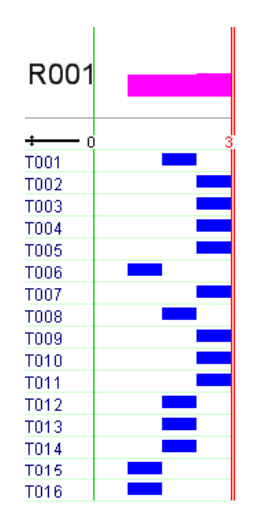
Fig. 13 Graphical representation of solution for the backup files model

Alternative formulation without scheduling

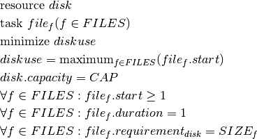
Instead of defining task and resource objects it is also possible to formulate this problem with a KCumulativeResourceConstraint constraint over standard finite domain variables that represent the different attributes of tasks without being grouped into a predefined object. A single KCumulativeResourceConstraint constraint expresses the problem of scheduling a set of tasks on one discrete resource by establishing the following relations between its arguments (five arrays of decision variables for the properties related to tasks start, duration, end, resource use and size all indexed by the same set and a constant or time-indexed resource capacity):

where UB stands for upper bound and LB for lower bound of a decision variable. Let savef denote the disk used for saving a file and the space used by the file (). As with scheduling objects, the start property of a task corresponds to the disk chosen for saving the file, and the resource requirement of a task is the file size. Since we want to save every file onto a single disk, the duration is fixed to 1. The remaining task properties end and size ( and ) that need to be provided in the formulation of cumulative constraints are not really required for our problem; their values are determined by the other three properties.

Implementation

The following model implements the second version using the cumulative constraint.

C++PythonJava

// Number of floppy disks
int  ND;
// Number of files
int NBFILES = 16;
// Floppy disk size
int CAP = 1440;
// Size of files to be saved
int SIZE[] = {46 ,55 ,62 ,87 ,108, 114, 137, 164, 253, 364, 372 ,388 ,406 ,432 ,461 ,851};
// index variable
int indexTask;
// Disk a file is saved on
KIntVarArray save;
// Space used by file on disk
KIntVarArray use;
// Auxiliary arrays for 'cumulative'
KIntVarArray dur,e,s;
// Number of disks used
KIntVar * diskuse;
// temporary array
KIntArray FSORT;

// Provide a sufficiently large number of disks
int sumsize = 0;
for (indexTask = 0;indexTask < NBFILES; indexTask++) {
    sumsize += SIZE[indexTask];
}
ND = ceil(sumsize / (float)(CAP));

// Creation of the problem in this session
KProblem problem(session,"D-4 Bin packing ");

char name[80];
// Setting up the tasks
for (indexTask = 0;indexTask < NBFILES; indexTask++) {
    sprintf(name,"save(%i)",indexTask);
    save += * ( new KIntVar( problem , name,0,ND-1 ) ) ;
    sprintf(name,"use(%i)",indexTask);
    use += * ( new KIntVar( problem , name,SIZE[indexTask],SIZE[indexTask]) );
    sprintf(name,"dur(%i)",indexTask);
    dur += * ( new KIntVar( problem , name,1,1) ) ;
    sprintf(name,"size(%i)",indexTask);
    s += * ( new KIntVar( problem , name,SIZE[indexTask],SIZE[indexTask]) ) ;
    sprintf(name,"end(%i)",indexTask);
    e += * ( new KIntVar( problem , name,1,ND) ) ;
}

diskuse = new KIntVar(problem,"diskuse",0,ND);

// Limit the number of disks used
problem.post(KMax("maxdisk",*diskuse,save));

// Capacity limit of disks
problem.post(KCumulativeResourceConstraint(problem ,save, e,dur, use, s, CAP));

// propagating problem
if (problem.propagate()) {
    printf("Problem is infeasible\n");
    exit(1);
}

// Definition of search strategy
KBranchingSchemeArray strategy;
strategy += KAssignVar(KSmallestMin(),KMinToMax(),save);

// Creation of the solver
KSolver solver(problem, strategy);

// minimize disk usage
problem.setSense(KProblem::Minimize);
problem.setObjective(*diskuse);

// Minimize the total number of disks used
int result = solver.optimize();

// solution printing
printf("Number of disks used: %f\n", problem.getSolution().getObjectiveValue()+1 );
int d;
for (d=0;d<=problem.getSolution().getObjectiveValue();d++) {
    printf("disk %i: ",d);
    int sumd = 0;
    for (indexTask = 0;indexTask < NBFILES; indexTask++) {
        if (problem.getSolution().getValue(save[indexTask]) == d) {
            printf("%i ",SIZE[indexTask]);
            sumd += SIZE[indexTask];
        }
    }
    printf("  space used: %i\n",sumd);
}

The solution produced by the execution of this model has the same objective function value, but the distribution of the files to the disks is not exactly the same: this problem has several different optimal solutions, in particular those that may be obtained be interchanging the order numbers of the disks. To shorten the search in such a case it may be useful to add some symmetry breaking constraints that reduce the size of the search space by removing a part of the feasible solutions. In the present example we may, for instance, assign the biggest file to the first disk and the second largest to one of the first two disks, and so on, until we reach a lower bound on the number of disks required (a safe lower bound estimate is given by rounding up to the next larger integer the sum of files sizes divided by the disk capacity).

Renewable and non-renewable resources

Besides the distinction disjunctive–cumulative or unary–discrete that we have encountered in the previous sections there are other ways of describing or classifying resources. Another important property is the concept of renewable versus non-renewable resources. The previous examples have shown instances of renewable resources (machine capacity, manpower etc.): the amount of resource used by a task is released at its completion and becomes available for other tasks. In the case of non-renewable resources (e.g. money, raw material, intermediate products), the tasks using the resource consume it, that is, the available quantity of the resource is diminuished by the amount used up by processing a task. Instead of using resources tasks may also produce certain quantities of resource. Again, we may have tasks that provide an amount of resource during their execution (renewable resources) or tasks that add the result of their production to a stock of resource (non-renewable resources).

Let us now see how to formulate the following problem: we wish to schedule five jobs P1 to P5 representing two stages of a production process. P1 and P2 produce an intermediate product that is needed by the jobs of the final stage (P3 to P5). For every job we are given its minimum and maximum duration, its cost or, for the jobs of the final stage, its profit contribution. There may be two cases, namely model A: the jobs of the first stage produce a given quantity of intermediate product (such as electricity, heat, steam) at every point of time during their execution, this intermediate product is consumed immediately by the jobs of the final stage. Model B: the intermediate product results as ouput from the jobs of the first stage and is required as input to start the jobs of the final stage. The intermediate product in model A is a renewable resource and in model B we have the case of a non-renewable resource.

Model formulation

Let 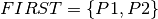be the set of jobs in the first stage, the jobs of the second stage, and the set the union of all jobs. For every job we are given its minimum and maximum duration and respectively. is the amount of resource needed as input or resulting as output from a job. Furthermore we have a cost for jobs of the first stage and a profit for jobs of the final stage.

Model A (renewable resource) : The case of a renewable resource is formulated by the following model. Notice that the resource capacity is set to 0 indicating that the only available quantities of resource are those produced by the jobs of the first production stage.

Model B (non-renewable resource) : In analogy to the model A we formulate the second case as follows.

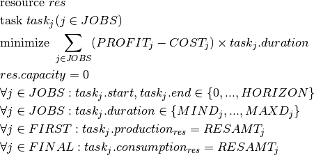
However, this model does not entirely correspond to the problem description above since the provision of the intermediate product occurs at the start of a task. To remedy this problem we may introduce an auxiliary task for every job in the first stage. The auxiliary job has duration 0, the same completion time as the original job and provides the intermediate product in the place of the original job.

Implementation

The following model implements case A. We use the default scheduling indicating by the value true for the optional second argument that we wish to maximize the objective function.

C++PythonJava

enum JOBS{P1,P2,P3,P4,P5};

char * names[] = {"P1","P2","P3","P4","P5"};

// Limits on job durations
int MIND[] = {3,4,0,4,10};
int MAXD[] = {15,26,15,25,20};

// Resource use/production
int RESAMT[] = {10,12,5,8,7};
// Time horizon
int HORIZON = 35;
// Profit from production
double PROFIT[] = {0,0,5.5,7,6.2};
// Cost of production
double COST[] = {1.8,1.6,0,0,0};
// Available resource quantity
int CAP = 0;

KFloatVar * totalProfit;

// Task objects for jobs
KTaskArray task;

// Non-renewable resource (intermediate prod.)
KDiscreteResource * intermProd;

// Creation of the problem in this session
KProblem problem(session,"Renewable resource");
// Creation of the schedule object with time horizon (0..HORIZON)
KSchedule schedule(problem,"Renewable resource schedule",0,HORIZON);


// Setting up the tasks
int indexJob;
for (indexJob = P1; indexJob <= P5; indexJob ++ ) {
    task += * ( new KTask(schedule, names[indexJob],0,HORIZON-MIND[indexJob],MIND[indexJob],MAXD[indexJob]) ) ;
    task[indexJob].getEndDateVar()->setSup(HORIZON);
}

// Setting up resources
intermProd = new KDiscreteResource(schedule,"IntP",CAP);

// Providing tasks
for (indexJob = P1; indexJob <= P2; indexJob ++ ) {
    task[indexJob].provides(*intermProd,RESAMT[indexJob]);
}

// Requiring tasks
for (indexJob = P3; indexJob <= P5; indexJob ++ ) {
    task[indexJob].requires(*intermProd,RESAMT[indexJob]);
}

// Objective function: total profit
totalProfit = new KFloatVar(problem,"totalProfit");
KLinTerm linTerm;
for (indexJob = P3; indexJob <= P5; indexJob ++ ) {
    linTerm = linTerm + PROFIT[indexJob] * (*task[indexJob].getDurationVar());
}
for (indexJob = P1; indexJob <= P5; indexJob ++ ) {
    linTerm = linTerm - COST[indexJob] * (*task[indexJob].getDurationVar());
}
problem.post(*totalProfit == linTerm);

// closing the schedule
schedule.close();

// propagating problem
if (problem.propagate()) {
    printf("Problem is infeasible\n");
    exit(1);
}

// maximizing totalProfit
schedule.setObjective(*totalProfit);
schedule.getProblem()->setSense(KProblem::Maximize);

schedule.setFunctionPointers(NULL,sfound,nfound,NULL,NULL,&problem);

// Find optimal schedule
int result = schedule.optimize();

// Solution printing
printf("Total profit: %f\n", problem.getSolution().getValue(*totalProfit));
printf("Job\tStart\tEnd\tDuration");
for (indexJob = P1; indexJob <= P5; indexJob ++ ) {
    printf("%i\t%i\t%i\t%i\n",indexJob, problem.getSolution().getValue(*task[indexJob].getStartDateVar()), problem.getSolution().getValue(*task[indexJob].getEndDateVar()), problem.getSolution().getValue(*task[indexJob].getDurationVar()));
}

The model for case B adds the two auxiliary tasks (forming the set ENDFIRST) that mark the completion of the jobs in the first stage. The only other difference are the task properties produces and consumes that define the resource constraints. We only repeat the relevant part of the model:

C++PythonJava

enum JOBS{P1,P2,endP1,endP2,P3,P4,P5};
char * names[] = {"P1","P2","endP1","endP2","P3","P4","P5"};

// Limits on job durations
int MIND[] = {3,4,0,1,1,4,10};
int MAXD[] = {15,26,1,1,15,25,20};

// Resource use/production
int RESAMT[] = {0,0,10,12,5,8,7};
// Time horizon
int HORIZON = 35;
// Profit from production
double PROFIT[] = {0,0,0,0,5.5,7,6.2};
// Cost of production
double COST[] = {1.8,1.6,0,0,0,0,0};
// Available resource quantity
int CAP = 0;

KFloatVar * totalProfit;

// Task objects for jobs
KTaskArray task;

// Non-renewable resource (intermediate prod.)
KDiscreteResource * intermProd;

// Creation of the problem in this session
KProblem problem(session,"Renewable resource (B)");
// Creation of the schedule object with time horizon (0..HORIZON)
KSchedule schedule(problem,"Renewable resource (B) schedule",0,HORIZON);


// Setting up the tasks
int indexJob;
for (indexJob = P1; indexJob <= P5; indexJob ++ ) {
    task += * ( new KTask(schedule, names[indexJob],0,HORIZON-MIND[indexJob],MIND[indexJob],MAXD[indexJob]) ) ;
    task[indexJob].getEndDateVar()->setSup(HORIZON);
}

// Setting up resources
intermProd = new KDiscreteResource(schedule,"IntP",CAP,false);

// Providing tasks
for (indexJob = endP1; indexJob <= endP2; indexJob ++ ) {
    task[indexJob].produces(*intermProd,RESAMT[indexJob]);
}

// Requiring tasks
for (indexJob = P3; indexJob <= P5; indexJob ++ ) {
    task[indexJob].consumes(*intermProd,RESAMT[indexJob]);
}


problem.post(*task[endP1].getStartDateVar() == *task[P1].getEndDateVar());
problem.post(*task[endP2].getStartDateVar() == *task[P2].getEndDateVar());

task[endP1].setDuration(1);
task[endP2].setDuration(1);

// Objective function: total profit
totalProfit = new KFloatVar(problem,"totalProfit");

KLinTerm linTerm;
for (indexJob = P3; indexJob <= P5; indexJob ++ ) {
    linTerm = linTerm + PROFIT[indexJob] * (*task[indexJob].getDurationVar());
}
for (indexJob = P1; indexJob <= P5; indexJob ++ ) {
    linTerm = linTerm - COST[indexJob] * (*task[indexJob].getDurationVar());
}
problem.post(*totalProfit == linTerm);

Results

The behavior of the (default) search and the results of the two models are considerably different. The optimal solution with an objective of 344.9 for case B represented in figure Fig. 15 is proven within a fraction of a second. Finding a good solution for case A takes several seconds on a standard PC; finding the optimal solution (see figure Fig. 14) and proving its optimality requires several minutes of running time. The main reason for this poor behavior of the search is our choice of the objective function: the cost-based objective function does not propagate well and therefore does not help with pruning the search tree. A better choice for objective functions in scheduling problems generally are criteria involving the task decision variables (start, duration, or completion time, particularly the latter).

Fig. 14 Solution for case A (resource provision and requirement)

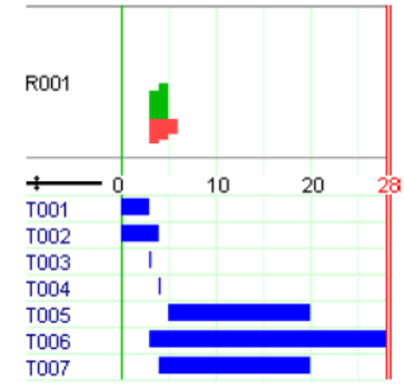
Fig. 15 Solution for case B (resource production and consumption)

Extensions: setup times

Consider once more the problem of planning the production of paint batches introduced in section Section 11.5. Between the processing of two batches the machine needs to be cleaned. The cleaning (or setup) times incurred are sequence-dependent and asymetric. The objective is to determine a production cycle of the shortest length.

Model formulation

For every job (), represented by a task object , we are given its processing duration . We also have a matrix of cleaning times with entries indicating the duration of the cleaning operation if task precedes task . The machine processing the jobs is modeled as a resource of unitary capacity, thus stating the disjunctions between the jobs.

With the objective to minimize the makespan (completion time of the last batch) we obtain the following model:

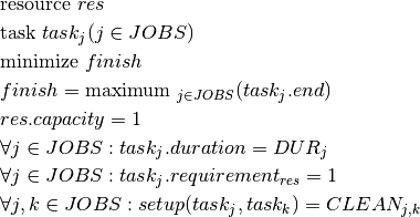
The tricky bit in the formulation of the original problem is that we wish to minimize the cycle time, that is, the completion of the last job plus the setup required between the last and the first jobs in the sequence. Since our task-based model does not contain any information about the sequence or rank of the jobs we introduce auxiliary variables and for the index values of the jobs in the first and last positions of the production cycle, and a variable for the duration of the setup operation between the last and first tasks. The following constraints express the relations between these variables and the task objects:

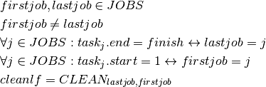
Minimizing the cycle time then corresponds to minimizing the sum .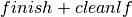

Implementation

The following model implements the task-based model formulated above. The setup times between tasks are set with the procedure KTask::setupTime() indicating the two task objects and the corresponding duration value.

C++PythonJava

// Number of paint batches (=jobs)
int NJ = 5;
// Durations of jobs
int DUR[]  = {40, 35, 45 ,32 ,50};

// Cleaning times between jobs
KIntMatrix CLEAN(5,5,0,"CLEAN");

CLEAN[0][0] = 0;CLEAN[1][0] = 11;CLEAN[2][0] = 7;CLEAN[3][0] = 13;CLEAN[4][0] = 11;
CLEAN[0][1] = 5;CLEAN[1][1] = 0;CLEAN[2][1] = 13;CLEAN[3][1] = 15;CLEAN[4][1] = 15;
CLEAN[0][2] = 13;CLEAN[1][2] = 15;CLEAN[2][2] = 0;CLEAN[3][2] = 23;CLEAN[4][2]= 11;
CLEAN[0][3] = 9;CLEAN[1][3] = 13;CLEAN[2][3] = 5;CLEAN[3][3] = 0;CLEAN[4][3] = 3;
CLEAN[0][4] = 3;CLEAN[1][4] = 7;CLEAN[2][4] = 7;CLEAN[3][4] = 7;CLEAN[4][4] = 0;

KTaskArray task;
KUnaryResource *res;

KIntVar * firstjob,*lastjob,*cleanlf,*finish;
KIntVarArray L;
// Objective variable
KIntVar * cycleTime;

// Creation of the problem in this session
KProblem problem(session,"B-5 Paint production");

// Creation of the schedule
KSchedule schedule(problem,"B-5 Paint production Schedule",0,10000);

// Setting up the resource (formulation of the disjunction of tasks)
res = new KUnaryResource(schedule,"res");

// Setting up the tasks
char name[80];
int j,i;
for (j=0;j<NJ;j++) {
    sprintf(name,"Task%i",j+1);
    task += (* new KTask(schedule,name,DUR[j],*res) );
    // Start times
    task[j].getStartDateVar()->setInf(1);
    L += *task[j].getEndDateVar();
}

for (j=0;j<NJ;j++) {
    for (i=j+1;i<NJ;i++) {
        task[i].setupTime(task[j],CLEAN[j][i],CLEAN[i][j]);
}
}

// Cleaning time at end of cycle (between last and first jobs)
firstjob = new KIntVar(problem,"firstjob",1,NJ);
lastjob  = new KIntVar(problem,"lastjob",1,NJ);
cleanlf  = new KIntVar(problem,"cleanlf",0,1000);
finish   = new KIntVar(problem,"finish",0,1000);

problem.post(*firstjob != *lastjob);

for (j=0;j<NJ;j++) {
    problem.post(  KEquiv( *task[j].getEndDateVar() == *schedule.getMakeSpan(), *lastjob == j+1)  );
    problem.post(  KEquiv( *task[j].getStartDateVar() == 1, *firstjob == j+1) );
}

// Cleaning time after every batch

KEltTerm2D kelt(CLEAN,*firstjob-1,*lastjob-1);
problem.post(new KElement2D(kelt,*cleanlf,"element"));

problem.post(new KMax("max",*finish,L) );

cycleTime   = new KIntVar(problem,"finish",0,1000);
// Objective: minimize the duration of a production cycle
problem.post( *cycleTime == *finish - 1 + *cleanlf ) ;

// Solve the problem
schedule.setFunctionPointers(NULL,sfound,NULL,NULL,NULL,&problem);
schedule.setObjective(*cycleTime);
int result = schedule.optimize();

// Solution printing
KIntArray SUCC;
for (j=0;j<NJ;j++) {
    SUCC += 0;
    for (i=0;i<NJ;i++) {
        if (problem.getSolution().getValue(*task[i].getStartDateVar()) == problem.getSolution().getValue(*task[j].getEndDateVar()) + CLEAN[i][j]) {
            SUCC[j] = i+1;
        }
    }
}
printf("Minimum cycle time: %i\n", problem.getSolution().getValue(*cycleTime));
printf("Sequence of batches:\nBatch\tStart\tDur\tCleaning\n");
for (i=0;i<NJ;i++) {
    printf(" %i\t%i\t%i\t%i\n",i
        ,problem.getSolution().getValue(*task[i].getStartDateVar())
        ,DUR[i]
        ,SUCC[i] > 0 ? CLEAN[SUCC[i]-1][i]: problem.getSolution().getValue(*cleanlf));
}

Results

The results are similar to those reported in Section 11.5 <kImplies>. It should be noted here that this model formulation is less efficient, in terms of search nodes and running times, than the previous model versions, and in particular the cycle constraint version presented in Section 11.7. However, the task-based formulation is more generic and easier to extend with additional features than the problem-specific formulations in the previous model versions.

The graphical representation as follows (figure Fig. 16).

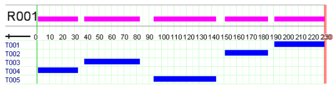
Fig. 16 Solution GANTT

Enumeration

In the previous scheduling examples we have used the default enumeration for scheduling problems, invoked by the optimization function KSchedule::optimize(). The built-in search strategies used by the solver in this case are particularly suited if we wish to minimize the completion time of a schedule. With other objectives the built-in strategies may not be a good choice, especially if the model contains decision variables that are not part of scheduling objects (the built-in strategies always enumerate first the scheduling objects). Artelys-Kalis makes it therefore possible to use the standard optimization function KSolver::optimize() in models that contain scheduling objects. The default search strategies employed by these optimization functions are different from the scheduling-specific ones and the user may also define his own problem specific enumeration as shown in the following examples.

User-defined enumeration strategies for scheduling problems may take two different forms: variable-based and task-based.

Task-based enumeration

A task-based enumeration strategy consists in the definition of a selection strategy choosing the task to be enumerated, a value selection heuristic for the task durations, and a value selection heuristic for the task start times.

Consider once more the problem of planning introduced in Section 12.5 . The behavior of the default scheduling strategy is very poor for this problem so we are going to define a custom search strategy tailored for this problem.

Implementation

The following model defines a taskbased branching strategy. We will use a two levels strategy:

• First select the task in the first set (because they are the one that provides resource) with the largest remaining domain for its duration variable and enumerate the possible values for this variable starting with the largest.

• Then select the other tasks (obtained via the method KSchedule::getTaskArray()) and apply the same task selection and value selection heuristics as in the first case

A task-based branching strategy is represented in Artelys-Kalis with the branching scheme KTaskSerializer. Several constructors are availables that takes as arguments the user or predefined task selection of type KTaskSelector, value selection strategies for the duration and start variables (standards KValueSelector), and a set of tasks it applies to (represented by the class KTaskArray). Such task-based branching strategies can be combined freely with any variable based branching strategies.

C++PythonJava

enum JOBS{P1,P2,P3,P4,P5};

char * names[] = {"P1","P2","P3","P4","P5"};

// Limits on job durations
int MIND[] = {3,4,0,4,10};
int MAXD[] = {15,26,15,25,20};

// Resource use/production
int RESAMT[] = {10,12,5,8,7};
// Time horizon
int HORIZON = 35;
// Profit from production
double PROFIT[] = {0,0,5.5,7,6.2};
// Cost of production
double COST[] = {1.8,1.6,0,0,0};
// Available resource quantity
int CAP = 0;

KFloatVar * totalProfit;

// Task objects for jobs
KTaskArray task;

// Non-renewable resource (intermediate prod.)
KDiscreteResource * intermProd;

// Creation of the problem in this session
KProblem problem(session,"Renewable resource");
// Creation of the schedule object with time horizon (0..HORIZON)
KSchedule schedule(problem,"Renewable resource schedule",0,HORIZON);


// Setting up the tasks
int indexJob;
for (indexJob = P1; indexJob <= P5; indexJob ++ ) {
    task += * ( new KTask(schedule, names[indexJob],0,HORIZON-MIND[indexJob],MIND[indexJob],MAXD[indexJob]) ) ;
    task[indexJob].getEndDateVar()->setSup(HORIZON);
}

// Setting up resources
intermProd = new KDiscreteResource(schedule,"IntP",CAP);

// Providing tasks
for (indexJob = P1; indexJob <= P2; indexJob ++ ) {
    task[indexJob].provides(*intermProd,RESAMT[indexJob]);
}

// Requiring tasks
for (indexJob = P3; indexJob <= P5; indexJob ++ ) {
    task[indexJob].requires(*intermProd,RESAMT[indexJob]);
}

// Objective function: total profit
totalProfit = new KFloatVar(problem,"totalProfit");
KLinTerm linTerm;
for (indexJob = P3; indexJob <= P5; indexJob ++ ) {
    linTerm = linTerm + PROFIT[indexJob] * (*task[indexJob].getDurationVar());
}
for (indexJob = P1; indexJob <= P5; indexJob ++ ) {
    linTerm = linTerm - COST[indexJob] * (*task[indexJob].getDurationVar());
}
problem.post(*totalProfit == linTerm);

// closing the schedule
schedule.close();

// propagating problem
if (problem.propagate()) {
    printf("Problem is infeasible\n");
    exit(1);
}

// maximizing totalProfit
schedule.setObjective(*totalProfit);
schedule.getProblem()->setSense(KProblem::Maximize);

schedule.setFunctionPointers(NULL,sfound,nfound,NULL,NULL,&problem);

if (!USE_DEFAULT_SCHEDULER) {

    KBranchingSchemeArray strategy;
    KTaskArray first;
    first += task[P1];
    first += task[P2];

    strategy += KTaskSerializer(first,&KLargestDurationDomain(),
                                  &KMaxToMin(),
                                  &KMaxToMin());

    strategy += KTaskSerializer(*schedule.getTaskArray(),
                                   &KLargestDurationDomain(),
                                   &KMaxToMin(),
                                   &KMaxToMin());

    schedule.setFirstSolutionSearchStrategy(strategy);
    schedule.setOptimalSolutionSearchStrategy(strategy);
}

// Find optimal schedule
int result = schedule.optimize();

// Solution printing
printf("Total profit: %f\n", problem.getSolution().getValue(*totalProfit));
printf("Job\tStart\tEnd\tDuration");
for (indexJob = P1; indexJob <= P5; indexJob ++ ) {
    printf("%i\t%i\t%i\t%i\n",indexJob,
             problem.getSolution().getValue(*task[indexJob].getStartDateVar()),
             problem.getSolution().getValue(*task[indexJob].getEndDateVar()),
             problem.getSolution().getValue(*task[indexJob].getDurationVar()));
}

Results

An optimal solution to this problem has an objective of 288.1. In comparison with the default scheduling strategy, our branching strategy reduces drastically the number of nodes that are enumerated and is able to prove optimality within a few seconds. A first solution is found immediately in 9 nodes with objective 281.9 and a second solution with a total profit of 288.1 if found in 8 more nodes. The scheduler enumerate then all the possibilities to prove optimality. Running the model results in the solution shown below:

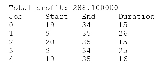
Fig. 17 Solution enumeration task-based

Multi-machines Disjunctive scheduling

Consider the typical definition of a job-shop scheduling problem: we are given a set of jobs that needs to be processed in a fixed order by a given set of machines. A machine executes one job at a time. The durations of the production tasks (= processing of a job on a machine) and the sequence of machines per job for a 6 × 6 instance are shown in following table. The objective is to minimize the makespan (latest completion time) of the schedule.

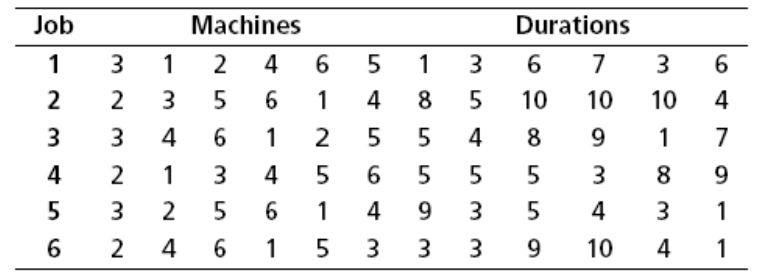
Fig. 18 6 x 6 Jobshop instance

Model formulation

Let denote the set of jobs and () the set of machines. Every job is produced as a sequence of tasks where needs to be finished before can start. A task is processed by the machine and has a fixed duration . The following model formulates the job-shop scheduling problem.

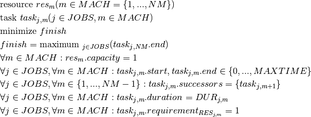
Implementation

The following model implements the job-shop scheduling problem:

C++PythonJava

// *** Modeling of the problem

// Creation of the problem in this session
KProblem problem(session,"JobShop CSP");
KSchedule s(problem,"JobShop Schedule",0,10000);


// Declaration and creation of the array keeping start dates of all tasks assigned to each job

KTask *** tasks = new KTask**[nbJobs];

KUnaryResource ** resources = new KUnaryResource*[nbRes];
int indexJob;
int indexRes;

for(indexRes = 0; indexRes < nbRes; indexRes++)
{
    char name[20];
    sprintf(name,"machine_%i",indexRes);
    resources[indexRes] = new KUnaryResource(s,name);
}

for (indexJob = 0; indexJob < nbJobs; indexJob++)
{
    tasks[indexJob] = new KTask*[nbRes];
    for(indexRes = 0; indexRes < nbRes; indexRes++)
    {
        char name[20];
        sprintf(name,"T%i_J%i",indexRes,indexJob);
        tasks[indexJob][indexRes] = new KTask(s,name,0,s.getTimeMax(),
                taskDuration[indexJob][indexRes],
                taskDuration[indexJob][indexRes]);
        tasks[indexJob][indexRes]->useResource(
            *resources[taskUse[indexJob][indexRes]],1);
    }
}

// constraints creation
for (indexJob = 0; indexJob < nbJobs; indexJob++)
{
    for(int indexRes = 0; indexRes < nbRes - 1; indexRes++)
    {
        //posting Precedence constraints between the tasks of a same JOB
        tasks[indexJob][indexRes+1]->startsAfter(*tasks[indexJob][indexRes]);
    }
}

s.setFunctionPointers(NULL,solution_found,NULL,NULL,NULL,&problem);
s.optimize();

// solution resume
s.getProblem()->getSolution().printResume();

Results

An optimal solution to this problem has a makespan of 55. A graphical representation of the solution is shown below:

Fig. 19 Solution GANTT

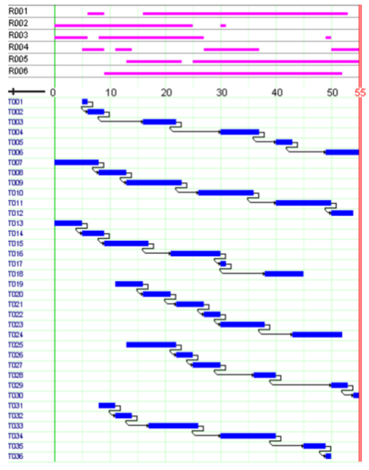
Resource usage

A resource usage is a means to specify the way that a resource will be produced / consumed / provided / required by a task. Three types of resource usages can be used:

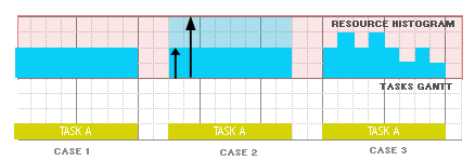
Fig. 20 Different resource usages

• case 1: Constant resource usage. This is the simplest case where the resource usage is constant all along the execution of the task. For example a task A will require 2 units of resource R during its execution.

• case 2: Variable resource usage but constant over the execution of the task. This case allows the resource usage to be variable but constant during the execution of the task. Therefore, a decision variable is associated with the resource usage that can be constrained like any other variable. For example a task A will require between 2 units and 4 units of resource R during its execution.

• case 3: Variable resource usage over the execution of the task. This case allows the resource usage to vary during the execution of the task using a resource usage profile defined as a KIntArray. For example, a task A will require [2,3,2,3,2,1,2,1] resource units wich means ’2’ for the first timestep of its execution; ’3’ for the second etc.. If the duration of the task exceeds the length of the profile, then the resource usage is considered as 0 after the end of the profile. If the task duration is smaller than the length of the profile, the profile will be truncated to the duration of the task.

Model formulation

Let be the set of tasks and the duration of . Let a resource of capacity required by all tasks for their execution and the resource usage profile of . With the objective of minimizing the makespan of the schedule we may formulate the model as follows.

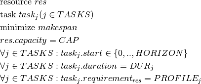
Implementation

The following model defines the explained model above, using a KResourceUsage to set the requirement constraint.

C++PythonJava

// Number of tasks
int nbTasks = 4;
// Duration of tasks
int duration[4] = { 7, 9, 8, 5 };
// Resource used profile per task
int profiles[][9] = { { 12, 12, 6, 2, 2, 2, 2 },
                              { 12, 12, 6, 2, 2, 2, 2, 2, 2 },
                              { 12, 12, 3, 3, 3, 3, 3, 3 },
                              { 6, 6, 6, 6, 6 } };
// Resource capacity
int resCapacity = 18;

// Creation of the problem in this session
KProblem problem(session, "Variable resource usage");

// Time horizon
int horizon = 0;
for (int dur : duration) {
    horizon += dur;
}
// Creation of the schedule object with time horizon (0..horizon)
KSchedule schedule(problem, "Variable resource usage schedule", 0, horizon);

// Tasks to be planned
KTaskArray tasks;

int indexTask;
// building each task with fixed duration
for (indexTask = 0; indexTask < nbTasks; indexTask++) {
    std::stringstream sout("");
    sout << "task_" << indexTask;
    tasks += KTask(schedule, sout.str().c_str(), duration[indexTask]);
}

// Creation of the resource
KDiscreteResource res(schedule, "resource", resCapacity);
// Requirement on the task indicating the resource usage
for (indexTask = 0; indexTask < nbTasks; indexTask++) {
    KIntArray profile_array;
    for (int step = 0; step < duration[indexTask]; step++) {
        profile_array += profiles[indexTask][step];
    }
    profile_array.print();
    tasks[indexTask].requires(KResourceUsage(res, profile_array));
}

// Minimize the makespan
schedule.optimize();
// solution printing
problem.getSolution().print();

Results

An optimal solution to this problem has a makespan of 11. A graphical representation of the solution is shown below where “Task a” represents task_1, “Task b” represents task_2, etc.

Fig. 21 Solution

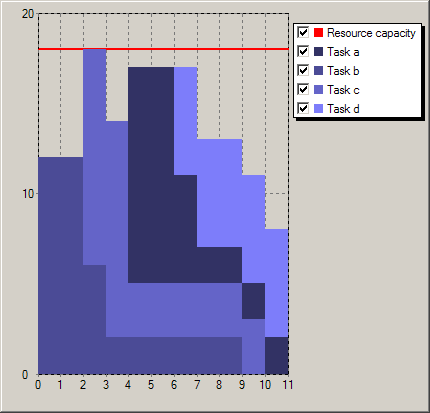
Branching strategy

When using KSchedule::optimize(), the search algorithm is decomposed in two distinct phases. The first phase targets the finding of an near optimal heuristic solution quickly. The second and last phase focuses on improving the bound and prove optimality. Thus, users have to specify the phase for which they set the custom branching scheme. They can set one for either phase or both phases.

In order to always have a meaningful branching scheme, some default strategies are implemented and used if no other branching strategy is defined in the model. These default strategies depend on the type of scheduling:

• Disjunctive scheduling: if all the resources used in the model are unary resources, then the default strategy for both phases is based on a KSettleDisjunction scheme (see Section 6.1). However if the unary resources are used as alternative resources, then the second default strategy used (see below).

• Cumulative scheduling: in this case, the default strategy for both phases uses a KAssignAndForbid (see Section 6.1) to set all the affectation variables on tasks and then a KTaskSerializer (see above) to instantiate the remaining tasks by instantiating their start and duration. The difference between the strategies of the first and second phase is in the KVariableSelector used in the KAssignAndForbid scheme. Indeed, during the first phase, a KRandomVariable is used whereas during the second phase, a KInputOrder is used.