Getting started with Python
How to set up the Knitro Python interface ?
The simplest way to set up the Knitro Python interface is to install the knitro Python package from PyPI using your preferred Python package manager:
pip install knitro
The package contains the Knitro binaries as well as the Python interface.
In a Python environment which has the knitro package installed,
you can either use Knitro through its Python interface
(by including import knitro in your Python code),
or call the solver from Pyomo with SolverFactory("knitroampl").
In order to use Knitro, you will need a valid license. If you do not yet have one, please visit http://www.artelys.com/knitro in order to obtain a trial license and start using Knitro.
Note
To generate a license, we often require an Artelys-specific identifier called the “machine-id”.
To know your machine-id, open a Python console in an environment with the Knitro package installed
and run: python -c "import knitro; knitro.KN_new()".
A message detailing your machine-id will appear near the top of the output.
If you are a legacy user and already have a working setup using Knitro binaries, you might prefer to setup the Python interface locally using your distribution: see section Setting up the Python interface from your Knitro distribution.
How to use the Knitro Python interface ?
The recommended way to use Knitro from Python is through the Problem class,
which allows writing optimization models in natural Python syntax.
It supports nonlinear models thanks to the Nonlinear Modeler, which provides
automatic differentiation.
For alternative interfaces (the knitro.optimize() single call interface for
large-scale models where API performance is critical, or the callable library for
fine-grained solver control), see the Knitro/Python reference.
Example
The following example solves the Rosenbrock problem (HS15), a classic nonlinear optimization test case:
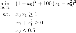
import knitro

with knitro.Problem() as prob:
    # Add the variables and set their bounds and initial values.
    x0 = prob.add_variable(ub=0.5, x0=-2.0)
    x1 = prob.add_variable(x0=1.0)

    # Add the constraints.
    prob.add_constraint(x0 * x1 >= 1.0)
    prob.add_constraint(x0 + x1**2 >= 0.0)

    # Set the objective.
    prob.add_objective(100.0 * (x1 - x0**2)**2 + (1.0 - x0)**2)

    # Set a solver parameter.
    prob.set_param("outlev", 4)

    # Solve the problem.
    status = prob.solve()
    print("x0 =", x0.value, "x1 =", x1.value)
Additional examples
More examples using the Python interface are provided in
the Python/examples directory of the Knitro distribution.