
struct Period
    price::Float64
    inflow::Float64
end

struct Turbine
    efficiency::Float64
    min_discharge::Float64
    max_discharge::Float64
    min_production::Float64
    max_production::Float64
end

struct Plant
    periods::Vector{Period}
    turbines::Vector{Turbine}
    min_volume::Float64
    max_volume::Float64
    initial_volume::Float64
    final_volume::Float64
    a_head::Float64
    b_head::Float64
    a_tail_q::Float64
    a_tail_s::Float64
    b_tail::Float64
end

function Plant(periods::Vector{Period}, turbines::Vector{Turbine})
    return Plant(
        periods, turbines, 5e6, 30e6, 25e6, 25e6, 1e-7, 50.0, 0.005, 0.001, 30.0
    )
end

num_periods(plant::Plant) = length(plant.periods)
num_turbines(plant::Plant) = length(plant.turbines)

struct Schedule
    revenue::Float64
    discharge::Vector{Vector{Float64}}
    production::Vector{Vector{Float64}}
    volume::Vector{Float64}
    headwater::Vector{Float64}
    tailwater::Vector{Float64}
    net_head::Vector{Float64}
endHydro Unit Commitment
Schedule the water discharge of several turbines sharing one reservoir to maximize the revenue from selling generated hydropower.
Introduction
Given a set of production units, the unit commitment problem consists in determining the status (on/off) of each unit at each period as well as the quantity of electricity to produce, in order to maximize the profit or satisfy demands while minimizing operational costs.
Here, we focus on hydropower generation.
The powerhouse contains a turbine and a generator. The water goes from the upstream reservoir to the downstream river through the penstock, passing by the powerhouse. The flow of water through the blades of a turbine generates electricity which is then transferred from the generator to its final destination through the long distance power lines. The water that passes through the penstock is used to generate power, but water could also be released from the reservoir directly to the downstream river. This water is said to be spilled, as it is not used for production, but rather to avoid an overflow of the reservoir.
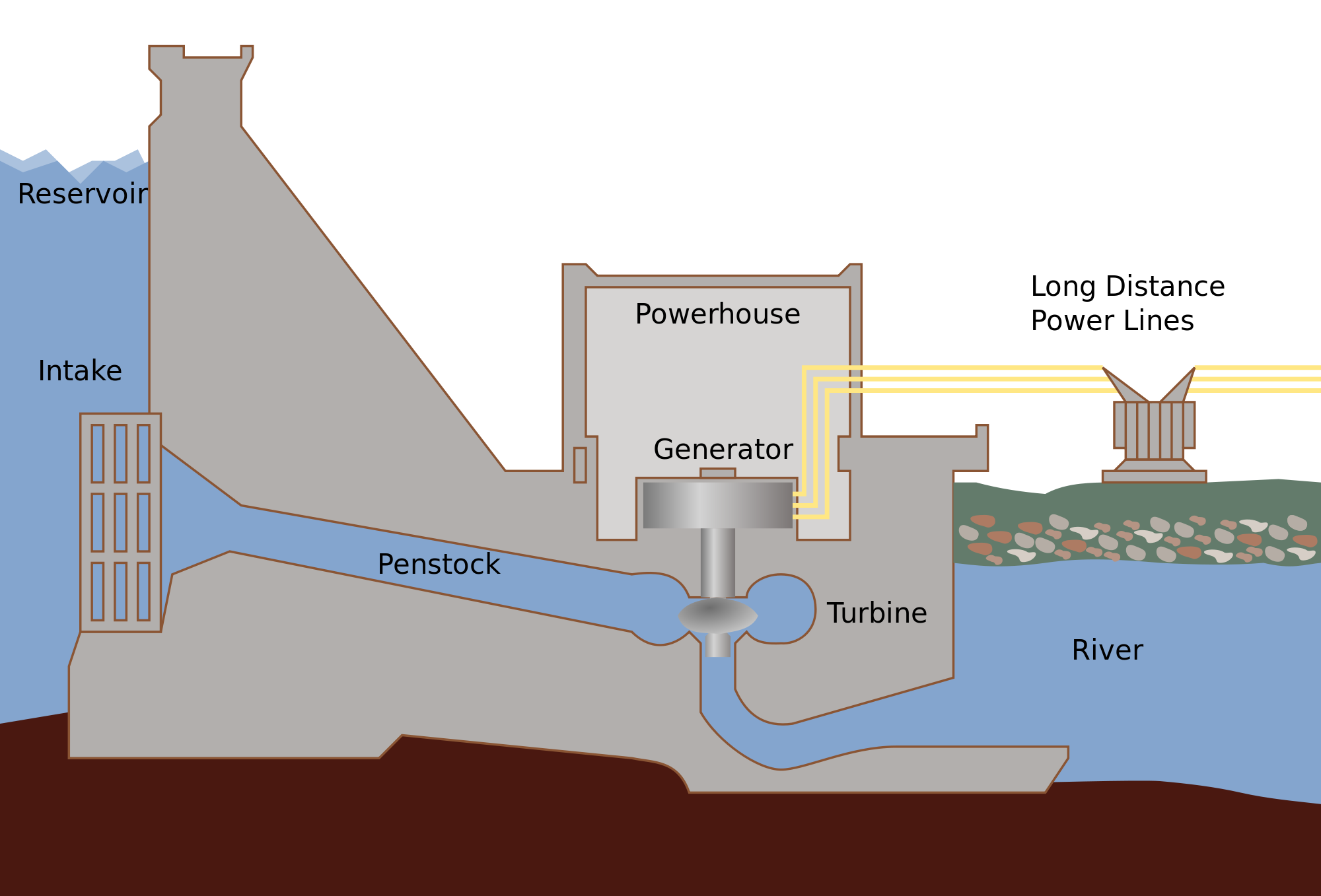
Image source: https://commons.wikimedia.org/wiki/File:Hydroelectric_dam-es.svg
How much electricity the water yields depends on how far it falls before reaching the turbine. That drop is measured between two water levels, the headwater of the upstream reservoir and the tailwater of the downstream river. Their difference is the net head, the effective height of the water column driving the turbine. Both levels move as the plant operates, the reservoir dropping as water leaves it and the river rising as discharged and spilled water arrive, so the net head changes from one period to the next.
The quantity of electricity \(p_{j, t}\) produced by turbine \(j\) at period \(t\) is a nonlinear function of the net head \(h^\text{net}_{t}\) and the water discharge \(q_{j,t}\):
\[ p_{j,t} = \eta_j \cdot q_{j,t} \cdot h^\text{net}_{t} \]
where \(\eta_j\) is called the efficiency of turbine \(j\), a coefficient that also carries the density of water, gravity and the conversion to megawatts.
That product of two variables is what makes the problem nonlinear, and it is also what ties the turbines together. They draw on one reservoir, so they share one net head, and water one of them discharges lowers what the others can produce later.
Problem description
Here, we consider a problem composed of several turbines and one reservoir. The objective is to maximize the revenue from selling generated power.
Input:
\(H\) periods; for each period \(t = 1, \dots, H\)
- a price \(R_t\) for selling a unit of electricity
- an inflow \(\Omega_t\)
\(N\) turbines; for each turbine \(j = 1, \dots, N\):
- a minimum discharge \(Q^\text{min}_j\)
- a maximum discharge \(Q^\text{max}_j\)
- a minimum production \(P^\text{min}_j\)
- a maximum production \(P^\text{max}_j\)
- an efficiency \(\eta_j\)
a minimum volume \(V^\text{min}\) for the reservoir
a maximum volume \(V^\text{max}\) for the reservoir
an initial volume \(V^\text{init}\) for the reservoir
a minimum final volume \(V^\text{final}\) for the reservoir
a function \(F^\text{head}(v) = A^\text{head} v + B^\text{head}\) that returns the headwater depending on the volume in the reservoir
a function \(F^\text{tail}(q, s) = A^\text{tail}_q q + A^\text{tail}_s s + B^\text{tail}\) that returns the tailwater depending on the water discharge and the spilled water
Problem: find the quantity of water to send through each turbine at each period such that:
The volume in the reservoir always stays in \([V^\text{min}, V^\text{max}]\)
The initial volume is equal to \(V^\text{init}\)
The final volume is greater than \(V^\text{final}\)
If a turbine is used
- the water discharge in this turbine belongs to \([Q^\text{min}, Q^\text{max}]\); otherwise, it is null.
- the production of this turbine belongs to \([P^\text{min}, P^\text{max}]\); otherwise, it is null.
Objective: maximize the revenue
Mixed-integer nonlinear program
Variables:
- \(x_{j, t} \in \{ 0, 1 \}\), \(j = 1, \dots, N\), \(t = 1, \dots, H\): \(x_{j, t} = 1\) iff turbine \(j\) is on at period \(t\), otherwise \(0\).
- \(q_{j, t} \in [0, Q_j^\text{max}]\), \(j = 1, \dots, N\), \(t = 1, \dots, H\): water discharge in turbine \(j\) at period \(t\).
- \(q^\text{tot}_t \in \mathbb{R}^+\), \(t = 1, \dots, H\): total water discharge at period \(t\).
- \(s_t \in \mathbb{R}^+\), \(t = 1, \dots, H\): water spilled at period \(t\).
- \(p_{j, t} \in [0, P_j^\text{max}]\), \(j = 1, \dots, N\), \(t = 1, \dots, H\): production of turbine \(j\) at period \(t\)
- \(v_t \in [V^\text{min}, V^\text{max}]\), \(t = 1, \dots, H\): volume in the reservoir at period \(t\)
- \(h^\text{head}_t \in \mathbb{R}\), \(t = 1, \dots, H\): head water at period \(t\)
- \(h^\text{tail}_t \in \mathbb{R}\), \(t = 1, \dots, H\): tail water at period \(t\)
- \(h^\text{net}_t \in \mathbb{R}^+\), \(t = 1, \dots, H\): net head at period \(t\)
Objective: maximize the revenue
\[ \max \sum_{t = 1}^H \sum_{j = 1}^N R_t p_{j, t} \]
Constraints:
- Initial and final volume:
\[ v_1 = V^\text{init} \]
\[ v_H \ge V^\text{final} \]
- Water balance: volume at \(t\) = volume at \(t - 1\) + inflow at \(t\) - consumption at \(t\). A period is one hour and the flows are per second, hence the factor 3600.
\[ \forall t = 2, \dots, H \qquad v_t = v_{t - 1} + 3600 \cdot \Omega_t - 3600 \cdot q^\text{tot}_t - 3600 \cdot s_t \]
- Water discharge limits
\[ \forall j = 1, \dots, N \quad \forall t = 1, \dots, H \qquad q_{j, t} \ge Q_j^\text{min} x_{j, t} \]
\[ \forall j = 1, \dots, N \quad \forall t = 1, \dots, H \qquad q_{j, t} \le Q_j^\text{max} x_{j, t} \]
- Production limits
\[ \forall j = 1, \dots, N \quad \forall t = 1, \dots, H \qquad p_{j, t} \ge P_j^\text{min} x_{j, t} \]
\[ \forall j = 1, \dots, N \quad \forall t = 1, \dots, H \qquad p_{j, t} \le P_j^\text{max} x_{j, t} \]
Both sides are gated by \(x_{j, t}\), so an idle turbine is held at zero discharge and zero production, and a running one is kept between its bounds.
- Total water discharge
\[ \forall t = 1, \dots, H \qquad q_t^\text{tot} = \sum_{j = 1}^N q_{j, t} \]
- Headwater
\[ \forall t = 1, \dots, H \qquad h_t^\text{head} = A^\text{head} v_t + B^\text{head} \]
- Tailwater
\[ \forall t = 1, \dots, H \qquad h_t^\text{tail} = A^\text{tail}_q q^\text{tot}_t + A^\text{tail}_s s_t + B^\text{tail} \]
- Net head
\[ \forall t = 1, \dots, H \qquad h_t^\text{net} = h_t^\text{head} - h_t^\text{tail} \]
- Hydropower production function
\[ \forall j = 1, \dots, N \quad \forall t = 1, \dots, H \qquad p_{j, t} = \eta_j \cdot q_{j,t} \cdot h^\text{net}_{t} \]
The model has the following properties:
- Continuous and binary variables
- Quadratic structures
- Non-convex
- Therefore, it is a non-convex MIQCQP
Input data
A Period carries what the horizon offers at one hour, the price a unit of electricity sells for and the inflow arriving at the reservoir. A Turbine carries its efficiency and the bounds it has to respect while it runs. A Plant holds those two lists plus everything that belongs to the reservoir rather than to any one turbine, namely the volume it must stay within, where it starts and where it has to end, and the coefficients of the two level functions.
A Schedule carries the revenue it earns, the discharge and production of every turbine at every period, and the four series the reservoir follows, namely volume, headwater, tailwater and net head.
The plant is generated rather than read from a file. Ten turbines draw on one reservoir over 168 hourly periods, a week of operation. Prices follow a daily cycle with noise on top, and the inflows are drawn flat. Each language draws with its own generator, so the plant scheduled here is not the one the Python pages schedule, and the two schedules cannot be compared hour by hour. _uniform and _triangular are here because the standard library has neither.
using Random

_uniform(rng, low, high) = low + (high - low) * rand(rng)

function _triangular(rng, low, high, mode)
    share = (mode - low) / (high - low)
    drawn = rand(rng)
    if drawn < share
        return low + sqrt(drawn * (high - low) * (mode - low))
    end
    return high - sqrt((1 - drawn) * (high - low) * (high - mode))
end

function generate_plant(periods_wanted, turbines_wanted)
    rng = MersenneTwister(periods_wanted * turbines_wanted)
    turbines = Turbine[]
    for _ in 1:turbines_wanted
        min_production = _uniform(rng, 0, 10)
        max_production = min_production + _uniform(rng, 0, 40)
        min_discharge = _triangular(rng, 0, 100, 10)
        max_discharge = _triangular(rng, min_discharge, 100, max(min_discharge, 90))
        push!(
            turbines,
            Turbine(
                _uniform(rng, 0.5, 0.9) * 1e-6 * 1000 * 9.81,
                min_discharge,
                max_discharge,
                min_production,
                max_production,
            ),
        )
    end
    periods = Period[]
    for t in 0:(periods_wanted - 1)
        inflow = _uniform(rng, 10, 100) * turbines_wanted
        cycle = 40 * (1 + cos(t / 24 * 2 * pi)) + 10
        push!(periods, Period(cycle + _uniform(rng, -10, 10), inflow))
    end
    return Plant(periods, turbines)
end

plant = generate_plant(168, 10)
Every figure is a stack of panels sharing one time axis, so a period reads straight down from one panel to the next. The discharge panel is a step area per turbine stacked into the total, since a turbine holds its discharge for the whole hour rather than sliding to the next value, and every other panel is a line.
Prices are the input the schedule reacts to, so they come first. The cycle is daily, and the noise on top is what keeps the schedule from being the same day repeated seven times.
draw_prices(plant)Model implementation
using JuMP
using KNITRO
maximize_revenue(plant) builds the model, solves it with Knitro, and returns a Schedule. The only nonlinear part is the production function, a product of two variables, so the same @constraint macro takes every line of the model. The turbine limits are constraints rather than variable bounds, because each side is gated by the on/off variable, so an idle turbine is pinned to zero.
Proving optimality on a nonconvex problem of this size takes far longer than reaching a good schedule, so the branch and bound stops at the first integer feasible point.
function maximize_revenue(
    plant::Plant; mip_terminate=KNITRO.KN_MIP_TERMINATE_FEASIBLE, num_threads=1
)
    H = num_periods(plant)
    N = num_turbines(plant)
    periods, turbines = plant.periods, plant.turbines

    model = Model(KNITRO.Optimizer)

    @variable(model, x[1:N, 1:H], Bin)
    @variable(model, q[1:N, 1:H] >= 0)
    @variable(model, p[1:N, 1:H] >= 0)
    @variable(model, qtot[1:H] >= 0)
    @variable(model, s[1:H] >= 0)
    @variable(model, plant.min_volume <= v[1:H] <= plant.max_volume)
    @variable(model, h_head[1:H])
    @variable(model, h_tail[1:H])
    @variable(model, h_net[1:H] >= 0)

    @objective(model, Max, sum(periods[t].price * p[j, t] for j in 1:N, t in 1:H))

    @constraint(
        model,
        [t in 2:H],
        v[t] == v[t - 1] + 3600 * (periods[t].inflow - qtot[t] - s[t])
    )

    for t in 1:H, j in 1:N
        turbine = turbines[j]
        @constraint(model, p[j, t] >= turbine.min_production * x[j, t])
        @constraint(model, p[j, t] <= turbine.max_production * x[j, t])
        @constraint(model, q[j, t] >= turbine.min_discharge * x[j, t])
        @constraint(model, q[j, t] <= turbine.max_discharge * x[j, t])
    end

    @constraint(model, [t in 1:H], qtot[t] == sum(q[j, t] for j in 1:N))
    @constraint(model, [t in 1:H], h_head[t] == plant.a_head * v[t] + plant.b_head)
    @constraint(
        model,
        [t in 1:H],
        h_tail[t] == plant.a_tail_q * qtot[t] + plant.a_tail_s * s[t] + plant.b_tail
    )
    @constraint(model, [t in 1:H], h_net[t] == h_head[t] - h_tail[t])
    @constraint(
        model,
        [t in 1:H, j in 1:N],
        p[j, t] == turbines[j].efficiency * q[j, t] * h_net[t]
    )

    @constraint(model, v[1] == plant.initial_volume)
    @constraint(model, v[H] >= plant.final_volume)
    @constraint(model, s[1] == 0)
    @constraint(model, [j in 1:N], q[j, 1] == 0)

    set_attribute(model, "mip_terminate", mip_terminate)
    set_attribute(model, "numthreads", num_threads)
    optimize!(model)

    revenue = objective_value(model)
    return Schedule(
        revenue,
        [[value(q[j, t]) for t in 1:H] for j in 1:N],
        [[value(p[j, t]) for t in 1:H] for j in 1:N],
        value.(v),
        value.(h_head),
        value.(h_tail),
        value.(h_net),
    )
end
schedule = maximize_revenue(plant);=======================================
Commercial License
Artelys Knitro 16.0.0
=======================================
Knitro changing mip_method from AUTO to 1.
No start point provided -- Knitro computing one.
Knitro presolve eliminated 537 variables (9%) and 568 constraints (6%) in 0.02s.
datacheck 0
feastol 1e-06
feastol_abs 1e-06
hessian_no_f 1
mip_terminate 1
numthreads 1
opttol 1e-06
opttol_abs 0.001
Knitro changing mip_root_nlpalg from AUTO to 1.
Knitro changing mip_node_nlpalg from AUTO to 1.
Knitro changing mip_branchrule from AUTO to 2.
Knitro changing mip_selectrule from AUTO to 2.
Knitro changing mip_mir from AUTO to 2.
Knitro changing mip_clique from AUTO to 0.
Knitro changing mip_zerohalf from AUTO to 0.
Knitro changing mip_liftproject from AUTO to 0.
Knitro changing mip_knapsack from AUTO to 2.
Knitro changing mip_gomory from AUTO to 0.
Knitro changing mip_cut_flowcover from AUTO to 2.
Knitro changing mip_cut_probing from AUTO to 1.
Knitro changing mip_rounding from AUTO to 3.
Knitro changing mip_heuristic_strategy from AUTO to 1.
Knitro changing mip_heuristic_feaspump from AUTO to 1.
Knitro changing mip_heuristic_misqp from AUTO to 0.
Knitro changing mip_heuristic_mpec from AUTO to 1.
Knitro changing mip_heuristic_diving from AUTO to 1926.
Knitro changing mip_heuristic_fixpropagate from AUTO to 62.
Knitro changing mip_heuristic_lns from AUTO to 0.
Knitro changing mip_heuristic_localsearch from AUTO to 1.
Knitro changing mip_pseudoinit from AUTO to 1.
WARNING: Problem appears to have nonlinear equalities and be non-convex.
The Knitro mixed integer solver is designed for convex problems.
For non-convex problems it is only a heuristic, and the reported
bounds and optimality claims cannot be verified.
Problem Characteristics | Presolved
-----------------------
Problem type: MIQCQP
Objective: maximize / linear
Number of variables: 6048 | 5511
bounds: lower upper range | lower upper range
3864 0 1848 | 3674 0 1835
free fixed | free fixed
336 0 | 2 0
cont. binary integer | cont. binary integer
4368 1680 0 | 3841 1670 0
Number of constraints: 9252 | 8684
eq. ineq. range | eq. ineq. range
linear: 851 6721 0 | 334 6680 0
quadratic: 1680 0 0 | 1670 0 0
Number of nonzeros:
objective Jacobian Hessian | objective Jacobian Hessian
linear: 1680 18993 | 1670 17867
quadratic: 0 3360 1680 | 0 3340 1670
total: 1680 22353 1680 | 1670 21207 1670
Knitro using Branch and Bound method with 1 thread.
Initial points
--------------
No initial point provided for the root node relaxation.
No primal point provided for the MIP.
Coefficient range:
linear objective: [1e+00, 1e+02] | [1e+00, 1e+02]
linear constraints: [1e-07, 4e+03] | [1e-06, 9e+01]
quadratic objective: [0e+00, 0e+00] | [0e+00, 0e+00]
quadratic constraints: [5e-03, 9e-03] | [5e-03, 9e-03]
variable bounds: [1e+00, 3e+07] | [1e+00, 3e+07]
constraint bounds: [3e+01, 2e+07] | [2e+01, 7e+03]
Root node relaxation
--------------------
Iter Objective Feasibility Optimality Time
error error (secs)
---- --------- ----------- ---------- ------
0 250723. 686.607 98.4671 0.115
1 252530. 686.603 13.5404 0.135
2 255326. 686.596 13.5404 0.148
3 257680. 686.587 13.5404 0.160
4 274883. 686.510 13.5404 0.173
5 309606. 686.271 16.4352 0.186
6 353744. 685.691 24.9905 0.199
7 459561. 681.651 44.7897 0.211
8 560579. 666.285 104.560 0.223
9 592867. 444.267 927.106 0.240
10 620436. 75.5757 537.662 0.262
11 629034. 19.5552 276.929 0.284
12 638761. 2.59524 231.030 0.306
13 655352. 1.40002 128.979 0.321
14 678577. 0.683617 46.0187 0.338
15 752836. 4.79827e-02 17.6571 0.359
16 793282. 1.24593e-02 4.10239 0.381
17 808083. 4.09193e-04 1.67473 0.402
18 814925. 1.01382e-02 0.982056 0.424
19 816938. 1.16727e-02 0.648086 0.445
20 817797. 4.72243e-03 0.330583 0.467
Root node cutting planes
------------------------
Iter Cuts Best solution Best bound Gap Time
value value (secs)
---- ---- ------------- ---------- --- ------
0 0 818151. FCRD inf 2.373
EXIT: Terminating at first integer feasible point.
HINT: The problem may be a non-convex mixed-integer problem. Set
mip_multistart=1 to enable a mixed-integer multistart heuristic,
which may improve the chances of finding the global solution.
Final Statistics for MIP
------------------------
Final objective value = 8.18150963729391224e+05
Final bound value = +inf
Final optimality gap (abs / rel) = inf / inf
# of root cutting plane rounds = 1
# of restarts = 0
# of nodes processed = 0 (0.679s)
# of strong branching evaluations = 0 (0.000s)
# of function evaluations = 0 (0.000s)
# of gradient evaluations = 0 (0.000s)
# of hessian evaluations = 0 (0.000s)
# of hessian-vector evaluations = 0
# of subproblems processed = 2 (2.295s)
Total program time (secs) = 2.37269 (2.369 CPU time)
Time spent in evaluations (secs) = 0.00000
Cuts statistics (gen / add)
---------------------------
Knapsack cuts = 0 / 0
Mixed-integer rounding cuts = 4 / 4
Flow-cover cuts = 0 / 0
Probing cuts = 0 / 0
Heuristics statistics (calls / successes / time)
------------------------------------------------
Feasibility pump = 0 / 0 / 0.000s
Rounding heuristic = 1 / 1 / 1.625s
MPEC heuristic = 0 / 0 / 0.000s
Local search heuristic = 0 / 0 / 0.000s
===========================================================================
Show the full outputHide the full output
Output visualization
What the schedule earns, and which turbines earn it:
report_schedule(plant, schedule)Revenue 818,151 over 168 hours
turbine hours on production revenue share
(MWh)
-----------------------------------------------
1 142 1,223 70,055 8.6%
2 116 1,018 65,983 8.1%
3 141 2,077 117,831 14.4%
4 125 1,494 92,426 11.3%
5 138 1,898 110,047 13.5%
6 129 1,665 100,883 12.3%
7 97 1,024 71,729 8.8%
8 146 1,862 102,935 12.6%
9 142 852 48,135 5.9%
10 69 490 38,128 4.7%
Reservoir 25.0M at the start, 25.0M at the end, 13.6M at its lowest
Net head 17.7m to 22.9m, so the same water is worth 1.30 times more at the top than at the bottomA turbine whose minimum production is more than its maximum discharge can reach at the heads the reservoir offers can never be switched on at all, so the model leaves it off for the whole week and it stands at zero hours in the table.
The schedule reads in five panels. They show the prices, the discharge of every turbine stacked into the total, the production summed over the turbines, the volume left in the reservoir, and the three water levels. Production tracks the price: the turbines run through the dear hours and idle through the cheap ones, refilling the reservoir while the water is worth less than it will be later. The levels follow. The headwater falls with the volume, the tailwater rises with what is discharged and spilled, and the net head, the gap between them, is what every unit of water is worth.
draw_schedule(plant, schedule)