Nonlinear Modeler

Overview

The Knitro Nonlinear Modeler allows describing expressions symbolically as expression trees. Once the expression is described, Knitro evaluates it and computes all required derivatives automatically using automatic differentiation (AD).

Note

The Nonlinear Modeler is currently available through the C and Python APIs only.

Introduction

Consider the following nonlinear program:

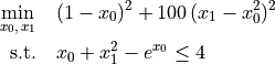
$\min_{x_0,\, x_1} \quad & (1 - x_0)^2 + 100\,(x_1 - x_0^2)^2\\ \text{s.t.} \quad & x_0 + x_1^2 - e^{x_0} \leq 4$

Both the objective and the constraint body are general nonlinear expressions. The Nonlinear Modeler represents each one as a directed acyclic graph (DAG), commonly referred to as an expression tree, in which every node is a mathematical operation and every leaf is either a variable or a numeric constant. Each intermediate node takes the values of its children as inputs; the root node’s value is the final result of the expression.

The expression trees for the objective $(1-x_0)^2 + 100\,(x_1 - x_0^2)^2$ and the constraint body 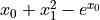$x_0 + x_1^2 - e^{x_0}$ are illustrated in the diagrams below:

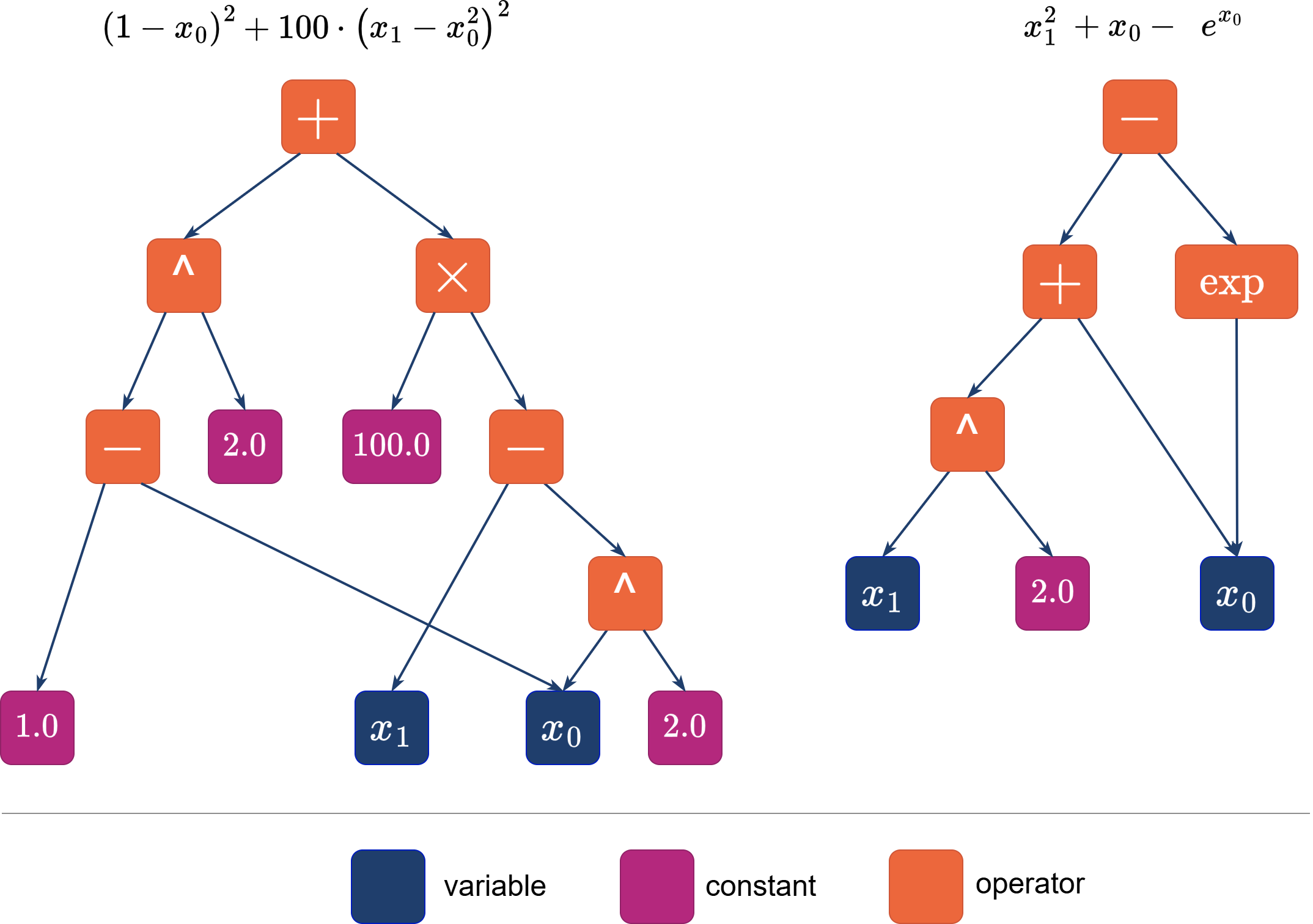
DAG of expression trees for the objective and constraint body

Expression trees are built bottom-up: starting from the leaves (variables and constants), combining them with operations to form sub-expressions, and continuing until the root is reached. The root is then passed to Knitro as an objective term or a constraint body term.

Available operations

The following operations are available to build expression trees.

Operator	Math notation	Type	Domain
Negation	$-x$	Unary	$x \in \mathbb{R}$
Sign	$\operatorname{sign}(x)$	Unary	$x \in \mathbb{R}$
Absolute value	$\|x\|$	Unary	$x \in \mathbb{R}$
Square root	$\sqrt{x}$	Unary	$x \geq 0$
Exponential	$e^x$	Unary	$x \in \mathbb{R}$
Exponential minus one	$e^x - 1$	Unary	$x \in \mathbb{R}$
Natural logarithm	$\ln x$	Unary	$x > 0$
Natural logarithm of $1+x$	$\ln(1+x)$	Unary	$x > -1$
Base-10 logarithm	$\log_{10} x$	Unary	$x > 0$
Sine	$\sin x$	Unary	$x \in \mathbb{R}$
Cosine	$\cos x$	Unary	$x \in \mathbb{R}$
Tangent	$\tan x$	Unary	$x \neq \tfrac{\pi}{2} + k\pi$
Arcsine	$\arcsin x$	Unary	$x \in [-1,\, 1]$
Arccosine	$\arccos x$	Unary	$x \in [-1,\, 1]$
Arctangent	$\arctan x$	Unary	$x \in \mathbb{R}$
Hyperbolic sine	$\sinh x$	Unary	$x \in \mathbb{R}$
Hyperbolic cosine	$\cosh x$	Unary	$x \in \mathbb{R}$
Hyperbolic tangent	$\tanh x$	Unary	$x \in \mathbb{R}$
Inverse hyperbolic sine	$\operatorname{arcsinh} x$	Unary	$x \in \mathbb{R}$
Inverse hyperbolic cosine	$\operatorname{arccosh} x$	Unary	$x \geq 1$
Inverse hyperbolic tangent	$\operatorname{arctanh} x$	Unary	$\|x\| < 1$
Error function	$\operatorname{erf}(x)$	Unary	$x \in \mathbb{R}$
Complementary error function	$\operatorname{erfc}(x)$	Unary	$x \in \mathbb{R}$
Addition	$a + b$	Binary	$a,\, b \in \mathbb{R}$
Subtraction	$a - b$	Binary	$a,\, b \in \mathbb{R}$
Multiplication	$a \times b$	Binary	$a,\, b \in \mathbb{R}$
Division	$a / b$	Binary	$a \in \mathbb{R},\; b \neq 0$
Power	$a^b$	Binary	$a > 0,\; b \in \mathbb{R}$
Two-argument arctangent	$\operatorname{atan2}(a, b)$	Binary	$(a, b) \neq (0, 0)$
Logarithm to an arbitrary base	$\log_b a$	Binary	$a > 0,\; b > 0,\; b \neq 1$
Sum of $n$ operands	$\sum_{i=1}^{n} a_i$	N-ary	$a_i \in \mathbb{R}$
Product of $n$ operands	$\prod_{i=1}^{n} a_i$	N-ary	$a_i \in \mathbb{R}$

C interface

Types

type KNVarId: An integer index that identifies a decision variable in the Knitro context. Variable indices are filled in by KN_add_vars when variables are added to the model.

type KNExprId: An integer handle that identifies a single expression node in the context. Every expression-builder function returns a KNExprId for the node it just created. The handle is then passed to other builder functions to compose larger expressions, or to KN_add_obj_expr / KN_add_con_expr to attach the finished tree to the model.

type KNConId: An integer index that identifies a constraint in the Knitro context. Constraint indices are filled in by KN_add_cons when constraints are added to the model, and are passed to KN_add_con_expr to associate an expression tree with a specific constraint.

Leaf expressions

Leaf nodes are the starting points of any expression tree. A leaf is either a variable or a numeric constant.

KN_var_expr

int KN_var_expr(KN_context *kc, KNVarId var, KNExprId *expr);
int KN_var_exprs(KN_context *kc, size_t n, const KNVarId *vars, KNExprId *exprs);

Return the expression handle(s) for the given variable(s). Most builder functions accept a KNVarId directly via the _v suffix (see below), which is usually more convenient than calling this function explicitly.

KN_constant_expr

int KN_constant_expr(KN_context *kc, double constant, KNExprId *expr);
int KN_constant_exprs(KN_context *kc, size_t n, const double *constants, KNExprId *exprs);

Return the expression handle(s) for the given numeric constant(s). Similarly, builder functions accept a double directly via the _c suffix.

Operand-type suffix convention

Rather than always converting variables and constants to expression handles first, builder functions accept operands of several types directly. The operand type is encoded in a suffix appended to the function name:

Suffix	Operand type(s)
(none)	`KNExprId` (the result of a previous expression)
`_v`	`KNVarId` (a variable index)
`_c`	`double` (a numeric constant)
`_vv`, `_vc`, `_cv`, `_cc`	Two operands: variable/variable, variable/constant, constant/variable, or constant/constant
`_xv`, `_vx`, `_xc`, `_cx`	An expression paired with a variable or a constant
`_xvc`	A heterogeneous mix of expressions, variables, and constants (n-ary only)

For example, KN_pow_expr_vc(kc, x0, 2.0, &result) computes $x_0^2$ where x0 is a KNVarId and 2.0 is a constant — no intermediate leaf-expression calls are needed.

Unary expressions

Each function below creates a new node applying a unary operation to a single operand. Three variants exist for every operator: the base name (operand is a KNExprId), the _v variant (operand is a KNVarId), and the _c variant (operand is a double).

All share the same signature pattern:

int KN_<op>_expr   (KN_context *kc, KNExprId operand, KNExprId *expr);
int KN_<op>_expr_v (KN_context *kc, KNVarId  operand, KNExprId *expr);
int KN_<op>_expr_c (KN_context *kc, double   operand, KNExprId *expr);

Operator	C function	Math notation
Negation	`KN_neg_expr`	$-x$
Sign	`KN_sign_expr`	$\operatorname{sign}(x)$
Absolute value	`KN_abs_expr`	$\|x\|$
Square root	`KN_sqrt_expr`	$\sqrt{x}$
Exponential	`KN_exp_expr`	$e^x$
Exponential minus one	`KN_expm1_expr`	$e^x - 1$
Natural logarithm	`KN_log_expr`	$\ln x$
Natural logarithm of $1+x$	`KN_log1p_expr`	$\ln(1+x)$
Base-10 logarithm	`KN_log10_expr`	$\log_{10} x$
Sine	`KN_sin_expr`	$\sin x$
Cosine	`KN_cos_expr`	$\cos x$
Tangent	`KN_tan_expr`	$\tan x$
Arcsine	`KN_asin_expr`	$\arcsin x$
Arccosine	`KN_acos_expr`	$\arccos x$
Arctangent	`KN_atan_expr`	$\arctan x$
Hyperbolic sine	`KN_sinh_expr`	$\sinh x$
Hyperbolic cosine	`KN_cosh_expr`	$\cosh x$
Hyperbolic tangent	`KN_tanh_expr`	$\tanh x$
Inverse hyperbolic sine	`KN_asinh_expr`	$\operatorname{arcsinh} x$
Inverse hyperbolic cosine	`KN_acosh_expr`	$\operatorname{arccosh} x$
Inverse hyperbolic tangent	`KN_atanh_expr`	$\operatorname{arctanh} x$
Error function	`KN_erf_expr`	$\operatorname{erf}(x)$
Complementary error function	`KN_erfc_expr`	$\operatorname{erfc}(x)$

Binary expressions

Each function below creates a node applying a binary operation to two operands. All operand-type suffixes are supported: _vv, _vc, _cv, _cc, _xv, _vx, _xc, _cx, and no suffix (both operands are KNExprId).

Example signatures:

/* both operands are KNExprId */
int KN_add_expr    (KN_context *kc, KNExprId left,  KNExprId right, KNExprId *expr);

/* variable base, constant exponent */
int KN_pow_expr_vc (KN_context *kc, KNVarId  base,  double   exp,   KNExprId *expr);

/* expression numerator, constant denominator */
int KN_div_expr_xc (KN_context *kc, KNExprId numer, double   denom, KNExprId *expr);

Operator	C function	Math notation
Addition	`KN_add_expr`	$a + b$
Subtraction	`KN_sub_expr`	$a - b$
Multiplication	`KN_mul_expr`	$a \times b$
Division	`KN_div_expr`	$a / b$
Power	`KN_pow_expr`	$a^b$
Two-argument arctangent	`KN_atan2_expr`	$\operatorname{atan2}(a, b)$
Logarithm to an arbitrary base	`KN_logb_expr`	$\log_b a$

N-ary expressions

When an operation involves more than two operands of the same kind, n-ary builders accept all operands at once, avoiding the need to chain binary operations.

The standard variants share this signature pattern:

int KN_<op>_expr    (KN_context *kc, size_t n, const KNExprId *operands, KNExprId *expr);
int KN_<op>_expr_v  (KN_context *kc, size_t n, const KNVarId  *operands, KNExprId *expr);
int KN_<op>_expr_c  (KN_context *kc, size_t n, const double   *operands, KNExprId *expr);

The _xvc variant accepts a heterogeneous mix of operand types in a single call:

int KN_<op>_expr_xvc(KN_context *kc,
                      size_t n_exprs,     const KNExprId *exprs,
                      size_t n_vars,      const KNVarId  *vars,
                      size_t n_constants, const double   *constants,
                      KNExprId *expr);

Operator	C function	Math notation
Sum of $n$ operands	`KN_nadd_expr`	$\sum_{i=1}^{n} a_i$
Product of $n$ operands	`KN_nmul_expr`	$\prod_{i=1}^{n} a_i$

Registering expressions with the model

Once the root of an expression tree has been built, it must be attached to the model before calling KN_solve.

KN_add_obj_expr

int KN_add_obj_expr(KN_context *kc, KNExprId expr);
int KN_add_obj_exprs(KN_context *kc, size_t n, const KNExprId *exprs);

Add one or more expression trees to the objective function. Multiple calls accumulate: every registered expression is summed to form the complete objective.

KN_add_con_expr

int KN_add_con_expr(KN_context *kc, KNConId con, KNExprId expr);
int KN_add_con_exprs(KN_context *kc, KNConId con, size_t n, const KNExprId *exprs);

Add one or more expression trees to the body of constraint con. The expression is summed with any linear or quadratic structure already loaded for that constraint.

Evaluating expressions

KN_evaluate_expr

int KN_evaluate_expr(KN_context *kc, KNExprId expr, const double *x, double *y);
int KN_evaluate_exprs(KN_context *kc, size_t n, const KNExprId *exprs, const double *x, double *y);
int KN_evaluate_exprs_all(KN_context *kc, const double *x, double *y);

Evaluate one, several, or all registered expression trees at the point x (an array of variable values of length equal to the number of variables in the model). If x is NULL, the current variable values stored in the context are used. Results are written to y. Knitro calls these functions internally during the solve; they are primarily useful for debugging or post-processing.

C examples

The following code builds the expression tree for the HS15 objective $100\,(x_1 - x_0^2)^2 + (1 - x_0)^2$ . The full example is available as examples/C/exampleNLP1AD.c.

/* Add two variables; KN_add_vars fills xIndex with their KNVarId values */
KNVarId xIndex[2];
KN_add_vars(kc, 2, xIndex);

/* x0^2 */
KNExprId x0sq;
KN_pow_expr_vc(kc, xIndex[0], 2.0, &x0sq);

/* x1 - x0^2 */
KNExprId x1_minus_x0sq;
KN_sub_expr_vx(kc, xIndex[1], x0sq, &x1_minus_x0sq);

/* (x1 - x0^2)^2 */
KNExprId x1_minus_x0sq_sq;
KN_pow_expr_xc(kc, x1_minus_x0sq, 2.0, &x1_minus_x0sq_sq);

/* 1 - x0 */
KNExprId one_minus_x0;
KN_sub_expr_cv(kc, 1.0, xIndex[0], &one_minus_x0);

/* (1 - x0)^2 */
KNExprId one_minus_x0_sq;
KN_pow_expr_xc(kc, one_minus_x0, 2.0, &one_minus_x0_sq);

/* 100*(x1 - x0^2)^2 */
KNExprId obj_expr;
KN_mul_expr_cx(kc, 100.0, x1_minus_x0sq_sq, &obj_expr);

/* 100*(x1 - x0^2)^2 + (1 - x0)^2  — root node */
KN_add_expr(kc, obj_expr, one_minus_x0_sq, &obj_expr);

/* Attach the root to the objective */
KN_add_obj_expr(kc, obj_expr);

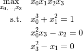
A second example, examples/C/exampleNLP2AD.c, models problem HS40 where the objective is a product of four variables — a natural fit for the n-ary KN_nmul_expr_v:

$\max_{x_0,\ldots,x_3} \quad & x_0 x_1 x_2 x_3 \\ \text{s.t.} \quad & x_0^3 + x_1^2 = 1 \\ & x_0^2 x_3 - x_2 = 0 \\ & x_3^2 - x_1 = 0$

/* Add four variables; KN_add_vars fills xIndex with their KNVarId values */
KNVarId xIndex[4];
KN_add_vars(kc, 4, xIndex);

/* Add three constraints; KN_add_cons fills cIndex with their KNConId values */
KNConId cIndex[3];
KN_add_cons(kc, 3, cIndex);

/* Objective: x0*x1*x2*x3 via n-ary product */
KNExprId obj_expr;
KN_nmul_expr_v(kc, 4, xIndex, &obj_expr);
KN_add_obj_expr(kc, obj_expr);

/* Constraint c0: x0^3 + x1^2 */
KNExprId x0_cubed, x1_sq, c0_expr;
KN_pow_expr_vc(kc, xIndex[0], 3.0, &x0_cubed);
KN_pow_expr_vc(kc, xIndex[1], 2.0, &x1_sq);
KN_add_expr(kc, x0_cubed, x1_sq, &c0_expr);
KN_add_con_expr(kc, cIndex[0], c0_expr);

examples/C/exampleMINLP1AD.c shows the same approach applied to a MINLP with binary variables and logarithmic expressions (KN_log1p_expr).

Python interface

The Problem class exposes the Nonlinear Modeler through Python operator overloading and a set of mathematical methods, so that expression trees can be written in natural mathematical notation without any API boilerplate.

Types and Problem methods

The full reference for the Python Nonlinear Modeler API — including types (Variable, Expression, Constraint, Relation, ComplementarityConstraint) and Problem methods — is available in the Knitro/Python reference.

Unary expressions

Unary operators are available either as Python operators applied directly to Variable and Expression objects, or as methods on the Problem instance. All methods accept an ExpressionLike and return an Expression.

Operator	Python expression	Math notation
Negation	`-x`	$-x$
Absolute value	`abs(x)`	$\|x\|$
Sign	`prob.sign(x)`	$\operatorname{sign}(x)$
Square root	`prob.sqrt(x)`	$\sqrt{x}$
Exponential	`prob.exp(x)`	$e^x$
Exponential minus one	`prob.expm1(x)`	$e^x - 1$
Natural logarithm	`prob.log(x)`	$\ln x$
Natural logarithm of $1+x$	`prob.log1p(x)`	$\ln(1+x)$
Base-10 logarithm	`prob.log10(x)`	$\log_{10} x$
Sine	`prob.sin(x)`	$\sin x$
Cosine	`prob.cos(x)`	$\cos x$
Tangent	`prob.tan(x)`	$\tan x$
Arcsine	`prob.asin(x)`	$\arcsin x$
Arccosine	`prob.acos(x)`	$\arccos x$
Arctangent	`prob.atan(x)`	$\arctan x$
Hyperbolic sine	`prob.sinh(x)`	$\sinh x$
Hyperbolic cosine	`prob.cosh(x)`	$\cosh x$
Hyperbolic tangent	`prob.tanh(x)`	$\tanh x$
Inverse hyperbolic sine	`prob.asinh(x)`	$\operatorname{arcsinh} x$
Inverse hyperbolic cosine	`prob.acosh(x)`	$\operatorname{arccosh} x$
Inverse hyperbolic tangent	`prob.atanh(x)`	$\operatorname{arctanh} x$
Error function	`prob.erf(x)`	$\operatorname{erf}(x)$
Complementary error function	`prob.erfc(x)`	$\operatorname{erfc}(x)$

Binary expressions

Binary operators are available either as Python operators on Variable and Expression objects, or as methods on the Problem instance.

Operator	Python expression	Math notation
Addition	`x + y`	$a + b$
Subtraction	`x - y`	$a - b$
Multiplication	`x * y`	$a \times b$
Division	`x / y`	$a / b$
Power	`x ** y`	$a^b$
Two-argument arctangent	`prob.atan2(y, x)`	$\operatorname{atan2}(a, b)$
Logarithm to an arbitrary base	`prob.log(x, base)`	$\log_b a$

N-ary expressions

N-ary operators are methods on the Problem instance. Each accepts either a single iterable or a variable number of ExpressionLike arguments.

Operator	Python expression	Math notation
Sum of $n$ operands	`prob.nsum(*args)`	$\sum_{i=1}^{n} a_i$
Product of $n$ operands	`prob.nprod(*args)`	$\prod_{i=1}^{n} a_i$

Python example

The same HS15 problem expressed with the Python interface:

import knitro

with knitro.Problem() as prob:
    x0 = prob.add_variable(ub=0.5, x0=-2.0)
    x1 = prob.add_variable(x0=1.0)

    prob.add_constraint(x0 * x1 >= 1.0)
    prob.add_constraint(x0 + x1**2 >= 0.0)

    prob.add_objective(100.0 * (x1 - x0**2)**2 + (1.0 - x0)**2)

    status = prob.solve()
    print("x0 =", x0.value, "x1 =", x1.value)

The arithmetic operators on Variable and Expression build the same tree shown in the Introduction section — the only difference is that the tree is described in Python syntax rather than with explicit API calls.

The following snippet shows add_complementarity_constraint for a simple complementarity pair $x \cdot y = 0$ , $x,y \geq 0$ :

import knitro

with knitro.Problem() as prob:
    x = prob.add_variable(lb=0.0)
    y = prob.add_variable(lb=0.0)

    prob.add_complementarity_constraint(x, y)

    prob.add_objective(x + y)
    prob.solve()

Interaction with callbacks

For most models, the Nonlinear Modeler suffices: expression trees are built, KN_solve (or prob.solve()) is called, and Knitro handles evaluation and differentiation automatically.

For advanced use cases, Knitro also provides a lower-level callback interface in which user-defined functions evaluate the objective and constraints. The two approaches can be mixed in the same model: some parts can be described as expression trees while others are handled by user callbacks. A new-point callback — a function Knitro calls every time it computes a new iterate — can always be registered alongside expression trees regardless of which approach is used for the model structure.