Evaluation callbacks
The evaluation callback interface registers callback functions that Knitro calls at each solver iteration to evaluate the nonlinear terms of the objective and constraints, together with their derivatives. This lower-level interface gives full control over function evaluation and differentiation, and is the natural choice when the model cannot easily be expressed as a symbolic tree or when hand-coded derivatives are available.
Tip
If the model is expressible using the built-in operators, consider the Nonlinear Modeler instead: expressions are described symbolically and Knitro computes all required derivatives automatically via automatic differentiation — no hand-written derivative code needed.
Applications should provide partial first derivatives whenever possible, to make Knitro more efficient and more robust. If first derivatives cannot be supplied, then the application should instruct Knitro to calculate finite-difference approximations.
First derivatives are represented by the gradient of the objective function and the Jacobian matrix of the constraints. Second derivatives are represented by the Hessian matrix, a linear combination of the second derivatives of the objective function and the constraints.
First derivatives
The default version of Knitro assumes that the user can provide exact first derivatives to compute the objective function gradient and constraint gradients. It is highly recommended that the user provide exact first derivatives if at all possible, since using first derivative approximations may seriously degrade the performance of the code and the likelihood of converging to a solution. However, if this is not possible the following first derivative approximation options may be used.
Forward finite-differences This option uses a forward finite-difference approximation of the objective and constraint gradients. The cost of computing this approximation is n function evaluations (where n is the number of variables). The option is invoked by choosing user option gradopt = 2.
Centered finite-differences This option uses a centered finite-difference approximation of the objective and constraint gradients. The cost of computing this approximation is 2n function evaluations (where n is the number of variables). The option is invoked by choosing user option gradopt = 3. The centered finite-difference approximation is often more accurate than the forward finite-difference approximation; however, it is more expensive to compute if the cost of evaluating a function is high.
Note
When using finite-difference gradients, the sparsity pattern for the constraint Jacobian should still be provided if possible to improve the efficiency of the finite-difference computation and decrease the memory requirements.
Although these finite-differences approximations should be avoided in general, they are useful to track errors: whenever the derivatives are provided by the user, it is useful to check that the differentiation (and the subsequent implementation of the derivatives) is correct. Indeed, providing derivatives that are not coherent with the function values is one of the most common errors when solving a nonlinear program. This check can be done automatically by comparing finite-differences approximations with user-provided derivatives. This is explained below (Checking derivatives).
Second derivatives
The default version of Knitro assumes that the application can provide exact second derivatives to compute the Hessian of the Lagrangian function. If the application is able to do so and the cost of computing the second derivatives is not overly expensive, it is highly recommended to provide exact second derivatives. However, Knitro also offers other options, which are described in detail below.
(Dense) Quasi-Newton BFGS:
The quasi-Newton BFGS option uses gradient information to compute a symmetric, positive-definite approximation to the Hessian matrix. Typically this method requires more iterations to converge than the exact Hessian version. However, since it is only computing gradients rather than Hessians, this approach may be more efficient in some cases. This option stores a dense quasi-Newton Hessian approximation so it is only recommended for small to medium problems (e.g., n < 1000). The quasi-Newton BFGS option is chosen by setting user option hessopt = 2.
(Dense) Quasi-Newton SR1:
As with the BFGS approach, the quasi-Newton SR1 approach builds an approximate Hessian using gradient information. However, unlike the BFGS approximation, the SR1 Hessian approximation is not restricted to be positive-definite. Therefore the quasi-Newton SR1 approximation may be a better approach, compared to the BFGS method, if there is a lot of negative curvature in the problem (i.e., the problem is not convex) since it may be able to maintain a better approximation to the true Hessian in this case. The quasi-Newton SR1 approximation maintains a dense Hessian approximation and so is only recommended for small to medium problems (e.g., n < 1000). The quasi-Newton SR1 option is chosen by setting user option hessopt = 3.
Finite-difference Hessian-vector product option:
If the problem is large and gradient evaluations are not a dominant cost, then Knitro can internally compute Hessian-vector products using finite-differences. Each Hessian-vector product in this case requires one additional gradient evaluation. This option is chosen by setting user option hessopt = 4. The option is only recommended if the exact gradients are provided.
Note
This option may not be used when nlp_algorithm = 1 or 4 since the Interior/Direct and SQP algorithms need the full expression of the Hessian matrix (Hessian-vector products are not sufficient).
Exact Hessian-vector products:
In some cases the application may prefer to provide exact Hessian-vector products, but not the full Hessian (for instance, if the problem has a large, dense Hessian). The application must provide a routine which, given a vector v (stored in hessVector), computes the Hessian-vector product, H*v, and returns the result (again in hessVector). This option is chosen by setting user option hessopt = 5.
Note
This option may not be used when nlp_algorithm = 1 or 4 since, as mentioned above, the Interior/Direct and SQP algorithms need the full expression of the Hessian matrix (Hessian-vector products are not sufficient).
Limited-memory Quasi-Newton BFGS:
The limited-memory quasi-Newton BFGS option is similar to the dense quasi-Newton BFGS option described above. However, it is better suited for large-scale problems since, instead of storing a dense Hessian approximation, it stores only a limited number of gradient vectors used to approximate the Hessian. The number of gradient vectors used to approximate the Hessian is controlled by user option lmsize.
A larger value of lmsize may result in a more accurate, but also more expensive, Hessian approximation. A smaller value may give a less accurate, but faster, Hessian approximation. When using the limited memory BFGS approach it is recommended to experiment with different values of this parameter (e.g. between 5 and 50).
In general, the limited-memory BFGS option requires more iterations to converge than the dense quasi-Newton BFGS approach, but will be much more efficient on large-scale problems. The limited-memory quasi-Newton option is chosen by setting user option hessopt = 6.
Note
When using a Hessian approximation option (i.e. hessopt > 1), you do not need to provide any sparsity pattern for the Hessian matrix since it is not used in the Hessian approximations. The Hessian sparsity pattern is only used when providing the exact Hessian (hessopt = 1).
As with exact first derivatives, exact second derivatives often provide a substantial benefit to Knitro and it is advised to provide them whenever possible. If the exact second derivative (i.e. the Hessian) matrix is provided by the user, it can (and should) be checked against a finite-difference approximation for errors using the Knitro derivative checker. See (Checking derivatives) below.
Jacobian and Hessian derivative matrices
The Jacobian matrix of the constraints is defined as

and the Hessian matrix of the Lagrangian is defined as
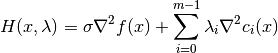
where  is the vector of Lagrange multipliers (dual variables),
and
is the vector of Lagrange multipliers (dual variables),
and  is a scalar (either 0 or 1) for the objective component of
the Hessian.
is a scalar (either 0 or 1) for the objective component of
the Hessian.
Note
For backwards compatibility
with older versions of Knitro, the user can always assume that
 if the user option hessian_no_f
=0 (which is the
default setting). However, if hessian_no_f=1, then Knitro will
provide a status flag to the user when it needs a Hessian evaluation
indicating whether the Hessian should be evaluated with
 or . The user must then evaluate the Hessian with
the proper value of based on this status flag.
Setting hessian_no_f
or . The user must then evaluate the Hessian with
the proper value of based on this status flag.
Setting hessian_no_f=1 and computing the Hessian with the requested
value of may improve Knitro efficiency in some cases.
Examples of how to do this can be found in the examples/C directory.
Example
Assume we want to use Knitro to solve the following problem:
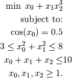
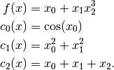
Rewriting in the Knitro standard notation, we have
Note
For demonstration purposes we show how to compute the Jacobian
and Hessian corresponding to all constraints and components of
this model. However, with the current API introduced in Knitro 11.0
the quadratic constraint  and the linear constraint
  should be loaded separately and should not be included in the
sparse Jacobian or Hessian structures provided through the nonlinear
callbacks. In addition, the linear term in the objective could
also be provided separately if desired.
should be loaded separately and should not be included in the
sparse Jacobian or Hessian structures provided through the nonlinear
callbacks. In addition, the linear term in the objective could
also be provided separately if desired.
Note
Please see the examples provided in examples/C/ which demonstrate
how to provide the derivatives (e.g. objective gradient, constraint Jacobian,
and Hessian) for nonlinear terms via callbacks for
different types of models, while loading linear and quadratic structures
separately.
Computing the Sparse Jacobian Matrix
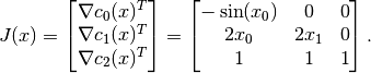
The gradients (first derivatives) of the objective and constraint functions are given by
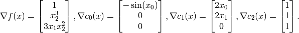
The constraint Jacobian matrix  is the matrix whose rows store the
(transposed) constraint gradients, i.e.,
is the matrix whose rows store the
(transposed) constraint gradients, i.e.,
The values of depend on the value of  and change during
the
solution process. The indices specifying the nonzero elements of this matrix
remain constant and are set in
and change during
the
solution process. The indices specifying the nonzero elements of this matrix
remain constant and are set in KN_set_cb_grad() by the values of
jacIndexCons and jacIndexVars.
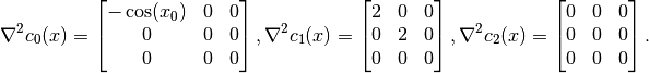
Computing the Sparse Hessian Matrix
For the example above, the Hessians (second derivatives) of the objective function is given by
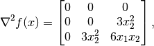
and the Hessians of constraints are given by
Scaling the objective matrix by , and the constraint matrices
by their corresponding Lagrange
multipliers and summing, we get
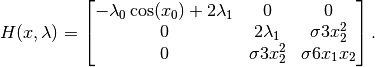
The values of  depend on the values of and
(and , which is either 0 or 1) and change during the
solution process. The indices specifying the nonzero elements of this matrix
remain constant and are set in
depend on the values of and
(and , which is either 0 or 1) and change during the
solution process. The indices specifying the nonzero elements of this matrix
remain constant and are set in KN_set_cb_hess() by the values of
hessIndexVars1 and hessIndexVars2.
Inputting derivatives
MATLAB users can provide the Jacobian and Hessian matrices in standard MATLAB format, either dense or sparse. See the fmincon documentation, http://www.mathworks.com/help/optim/ug/writing-constraints.html#brhkghv-16, for more information. Users of the callable library must provide derivatives to Knitro in sparse format. In the above example, the number of nonzero elements nnzJ in J(x) is 6, and these arrays would be specified as follows (here in column-wise order, but the order is arbitrary) using the callable library.
jac[0] = -sin(x[0]);  jacIndexCons[0] = 0; jacIndexVars[0] = 0;
jac[1] = 2*x[0];      jacIndexCons[1] = 1; jacIndexVars[1] = 0;
jac[2] = 1;           jacIndexCons[2] = 2; jacIndexVars[2] = 0;
jac[3] = 2*x[1];      jacIndexCons[3] = 1; jacIndexVars[3] = 1;
jac[4] = 1;           jacIndexCons[4] = 2; jacIndexVars[4] = 1;
jac[5] = 1;           jacIndexCons[5] = 2; jacIndexVars[5] = 2;
In the object-oriented interface, these values are set in the user-defined problem class by implementing a
non-zero pattern for the Jacobian sparse matrix, and providing jacIndexCons and jacIndexVars values
setJacNnzPattern({ {0, 1, 2, 1, 2, 2}, {0, 0, 0, 1, 1, 2} });
Note
Using KNProblem class, by default the Jacobian is assumed to be dense
and stored row-wise.
Note
Even if the application does not evaluate derivatives (i.e. finite-difference first derivatives are used), it must still provide a sparsity pattern for the constraint Jacobian matrix that specifies which partial derivatives are nonzero. Knitro uses the sparsity pattern to speed up linear algebra computations.
Note
When using finite-difference first derivatives (gradopt > 1),
if the sparsity pattern is unknown, then the application should specify a
fully dense pattern (i.e., assume all partial derivatives are nonzero).
This can easily and automatically be done by setting nnzJ to either
KN_DENSE_ROWMAJOR or KN_DENSE_COLMAJOR in the callable
library function KN_set_cb_grad()
(and setting jacIndexCons and jacIndexVars to be NULL).
Since the Hessian matrix will always be a symmetric matrix, Knitro only stores the nonzero elements corresponding to the upper triangular part (including the diagonal). In the example here, the number of nonzero elements in the upper triangular part of the Hessian matrix nnzH is 4. The Knitro array hess stores the values of these elements, while the arrays hessIndexVars1 and hessIndexVars2 store the row and column indices respectively. The order in which these nonzero elements is stored is not important. If we store them row-wise, the arrays hess, hessIndexVars1 and hessIndexVars2 are as follows:
hess[0] = -lambda[0]*cos(x[0]) + 2*lambda[1];
hessIndexVars1[0] = 0;
hessIndexVars2[0] = 0;

hess[1] = 2*lambda[1];
hessIndexVars1[1] = 1;
hessIndexVars2[1] = 1;

hess[2] = sigma*3*x[2]*x[2];
hessIndexVars1[2] = 1;
hessIndexVars2[2] = 2;

hess[3] = sigma*6*x[1]*x[2];
hessIndexVars1[3] = 2;
hessIndexVars2[3] = 2;
In the object-oriented interface, these values are set in the user-defined problem class by implementing a
non-zero pattern for the Hessian sparse matrix, and providing hessIndexRows and hessIndexCols values:
setHessNnzPattern({ {0, 1, 1, 2}, {0, 1, 2, 2} });
Note
In Knitro, the array objGrad corresponding to
 , can be provided in dense or sparse form.
The arrays jac, jacIndexCons, and
jacIndexVars store information concerning only the nonzero
(and typically nonlinear) elements of J(x). The array jac stores the nonzero values in
J(x) evaluated at the current solution estimate x,
jacIndexCons stores the constraint function (or row) indices
corresponding to these values, and jacIndexVars stores the variable
(or column) indices. There is no
restriction on the order in which these elements are stored; however,
it is common to store the nonzero elements of J(x) in either row-wise
or column-wise fashion.
, can be provided in dense or sparse form.
The arrays jac, jacIndexCons, and
jacIndexVars store information concerning only the nonzero
(and typically nonlinear) elements of J(x). The array jac stores the nonzero values in
J(x) evaluated at the current solution estimate x,
jacIndexCons stores the constraint function (or row) indices
corresponding to these values, and jacIndexVars stores the variable
(or column) indices. There is no
restriction on the order in which these elements are stored; however,
it is common to store the nonzero elements of J(x) in either row-wise
or column-wise fashion.
MATLAB example
Let us modify our example from Getting started with MATLAB so that the first derivatives are provided as well. In MATLAB, you only need to provide the derivatives for the nonlinear functions. In the example below, only the inequality constraint is nonlinear, so we only provide the derivative for this constraint.
function firstDer()

        function [f, g] = obj(x)
                f = 1000 - x(1)^2 - 2*x(2)^2 - x(3)^2 - x(1)*x(2) - x(1)*x(3);
                if nargout == 2
                   g = [-2*x(1) - x(2) - x(3); - 4*x(2) - x(1); -2*x(3) - x(1)];
                end
        end

        % nlcon should return [c, ceq, GC, GCeq]
        % with c(x) <= 0 and ceq(x) = 0
        function [c, ceq, GC, GCeq] = nlcon(x)
                c = -(x(1)^2 + x(2)^2 + x(3)^2 - 25);
                ceq = [];
                if nargout==4
                        GC = -([2*x(1); 2*x(2); 2*x(3)]);
                        GCeq = [];
                end
        end

        x0  = [2; 2; 2];
        A = []; b = []; % no linear inequality constraints ("A*x <= b")
        Aeq = [8 14 7]; beq = [56]; % linear equality constraints ("Aeq*x = beq")
        lb = zeros(3,1); ub = []; % lower and upper bounds

        options = knitro_options('gradopt', 1);
        knitro_nlp(@obj, x0, A, b, Aeq, beq, lb, ub, @nlcon, [], options);

end
The only difference with the derivative-free case is that the code that computes the objective function and the constraints also returns the first derivatives along with function values. The output is as follows.
=======================================
          Commercial License
         Artelys Knitro 16.0.0
=======================================

Knitro presolve eliminated 0 variables and 0 constraints.

concurrent_evals:        0
feastol                  1e-06
feastol_abs              0.001
opttol                   1e-06
opttol_abs               0.001

Problem Characteristics                     |           Presolved
-----------------------
Problem type: NLP
Objective: minimize / general
Number of variables:                      3 |                             3
  bounds:         lower     upper     range |     lower     upper     range
                      3         0         0 |         3         0         0
                             free     fixed |                free     fixed
                                0         0 |                   0         0
Number of constraints:                    2 |                             2
                    eq.     ineq.     range |       eq.     ineq.     range
  linear:             1         0         0 |         1         0         0
  quadratic:          0         0         0 |         0         0         0
  nonlinear:          0         1         0 |         0         1         0
Number of nonzeros:
              objective  Jacobian   Hessian | objective  Jacobian   Hessian
  linear:             0         3           |         0         3
  quadratic:          0         0         0 |         0         0         0
  nonlinear:          3         3         0 |         3         3         0
  total:              3         6         0 |         3         6         6
Coefficient range:
  linear objective:          [0e+00, 0e+00] |                [0e+00, 0e+00]
  linear constraints:        [7e+00, 1e+01] |                [7e+00, 1e+01]
  quadratic objective:       [0e+00, 0e+00] |                [0e+00, 0e+00]
  quadratic constraints:     [0e+00, 0e+00] |                [0e+00, 0e+00]
  variable bounds:           [0e+00, 0e+00] |                [0e+00, 0e+00]
  constraint bounds:         [6e+01, 6e+01] |                [6e+01, 6e+01]

Knitro using the Interior-Point/Barrier Direct algorithm.

    Iter       Objective  FeasError   OptError   ||Step||      Time
--------  --------------  ---------  ---------  ---------  --------
       0    9.760000e+02   1.30e+01
       8    9.360000e+02   0.00e+00   5.60e-08   2.36e-08      0.00


EXIT: Locally optimal solution found.

Final Statistics
----------------
Final objective value               =   9.36000000000080e+02
Final feasibility error (abs / rel) =   0.00e+00 / 0.00e+00
Final optimality error  (abs / rel) =   5.60e-08 / 3.50e-09
# of iterations                     =          8
# of CG iterations                  =          0
# of function evaluations           =         11
# of gradient evaluations           =         11
Total program time (secs)           =       0.00319 (     0.005 CPU time)
Time spent in evaluations (secs)    =       0.00183

===============================================================================
The number of function evaluation was reduced to 11, simply by providing exact first derivatives. This small example shows the practical importance of being able to provide exact derivatives.
C/C++ example
Let us show how to provide derivatives through the callable library API. Here we
look at the C example examples/C/exampleNLP2.c, which solves the model:
max   x0*x1*x2*x3         (obj)
s.t.  x0^3 + x1^2 = 1     (c0)
      x0^2*x3 - x2 = 0    (c1)
      x3^2 - x1 = 0       (c2)
Note that this problem has linear terms, quadratic terms and general nonlinear terms. We will show how to provide both first and second derivatives for the nonlinear structure through callbacks while separately loading the linear and quadratic structure.
#include <stdio.h>
#include <stdlib.h>
#include "knitro.h"


/** Callback for nonlinear function evaluations */
int callbackEvalFC (KN_context_ptr             kc,
                    CB_context_ptr             cb,
                    KN_eval_request_ptr const  evalRequest,
                    KN_eval_result_ptr  const  evalResult,
                    void              * const  userParams)
{
    const double *x;
    double *obj;
    double *c;

    if (evalRequest->type != KN_RC_EVALFC)
    {
        printf ("*** callbackEvalFC incorrectly called with eval type %d\n",
                evalRequest->type);
        return( -1 );
    }
    x = evalRequest->x;
    obj = evalResult->obj;
    c = evalResult->c;

    /** Evaluate nonlinear term in objective */
    *obj = x[0]*x[1]*x[2]*x[3];

    /** Evaluate nonlinear terms in constraints */
    c[0] = x[0]*x[0]*x[0];
    c[1] = x[0]*x[0]*x[3];

    return( 0 );
}

/** Callback for nonlinear gradient/Jacobian evaluations */
int callbackEvalGA (KN_context_ptr             kc,
                    CB_context_ptr             cb,
                    KN_eval_request_ptr const  evalRequest,
                    KN_eval_result_ptr  const  evalResult,
                    void              * const  userParams)
{
    const double *x;
    double *objGrad;
    double *jac;

    if (evalRequest->type != KN_RC_EVALGA)
    {
        printf ("*** callbackEvalGA incorrectly called with eval type %d\n",
                evalRequest->type);
        return( -1 );
    }
    x = evalRequest->x;
    objGrad = evalResult->objGrad;
    jac = evalResult->jac;

    /** Evaluate nonlinear term in objective gradient */
    objGrad[0] = x[1]*x[2]*x[3];
    objGrad[1] = x[0]*x[2]*x[3];
    objGrad[2] = x[0]*x[1]*x[3];
    objGrad[3] = x[0]*x[1]*x[2];

    /** Evaluate nonlinear terms in constraint gradients (Jacobian) */
    jac[0] = 3.0*x[0]*x[0]; /* derivative of x0^3 term  wrt x0    */
    jac[1] = 2.0*x[0]*x[3]; /* derivative of x0^2*x3 term  wrt x0 */
    jac[2] = x[0]*x[0];     /* derivative of x0^2*x3 terms wrt x3 */

    return( 0 );
}

/** Callback for nonlinear Hessian evaluation */
int callbackEvalH (KN_context_ptr             kc,
                   CB_context_ptr             cb,
                   KN_eval_request_ptr const  evalRequest,
                   KN_eval_result_ptr  const  evalResult,
                   void              * const  userParams)
{
    const double *x;
    const double *lambda;
    double sigma;
    double *hess;

    if (   evalRequest->type != KN_RC_EVALH
        && evalRequest->type != KN_RC_EVALH_NO_F )
    {
        printf ("*** callbackEvalHess incorrectly called with eval type %d\n",
                evalRequest->type);
        return( -1 );
    }

    x = evalRequest->x;
    lambda = evalRequest->lambda;
    /** Scale objective component of the Hessian by sigma */
    sigma = *(evalRequest->sigma);
    hess = evalResult->hess;

    /** Evaluate nonlinear term in the Hessian of the Lagrangian */
    hess[0] = lambda[0]*6.0*x[0] + lambda[1]*2.0*x[3];
    hess[1] = sigma*x[2]*x[3];
    hess[2] = sigma*x[1]*x[3];
    hess[3] = sigma*x[1]*x[2] + lambda[1]*2.0*x[0];
    hess[4] = sigma*x[0]*x[3];
    hess[5] = sigma*x[0]*x[2];
    hess[6] = sigma*x[0]*x[1];

    return( 0 );
}

/** main function */
int  main (int  argc, char  *argv[])
{
    int  i, nStatus, error;

    /** Declare variables. */
    KN_context   *kc;
    int    n, m;
    double cEqBnds[3] = {1.0, 0.0, 0.0};
    /** Used to define linear constraint structure */
    int    lconIndexCons[2];
    int    lconIndexVars[2];
    double lconCoefs[2];
    /** Used to define quadratic constraint structure */
    int    qconIndexCons[2];
    int    qconIndexVars1[2];
    int    qconIndexVars2[2];
    double qconCoefs[2];
    /** Pointer to structure holding information for nonlinear
     *  evaluation callback for terms:
     *     x0*x1*x2*x3  in the objective
     *     x0^3         in first constraint
     *     x0^2*x3      in second constraint */
    CB_context   *cb;
    int    cIndices[2];
    /** Used to define Jacobian structure for nonlinear terms
     *  evaluated in the callback. */
    int    cbjacIndexCons[3];
    int    cbjacIndexVars[3];
    double cbjacCoefs[3];
    /** Used to define Hessian structure for nonlinear terms
     *  evaluated in the callback. */
    int    cbhessIndexVars1[7];
    int    cbhessIndexVars2[7];
    double cbhessCoefs[7];
    /** For solution information */
    double x[4];
    double objSol;
    double feasError, optError;

    /** Create a new Knitro solver instance. */
    error = KN_new(&kc);
    if (error) exit(-1);
    if (kc == NULL)
    {
        printf ("Failed to find a valid license.\n");
        return( -1 );
    }

    /** Initialize Knitro with the problem definition. */

    /** Add the variables and specify initial values for them.
     *  Note: any unset lower bounds are assumed to be
     *  unbounded below and any unset upper bounds are
     *  assumed to be unbounded above. */
    n = 4;
    error = KN_add_vars(kc, n, NULL);
    if (error) exit(-1);
    for (i=0; i<n; i++) {
        error = KN_set_var_primal_init_value(kc, i, 0.8);
        if (error) exit(-1);
    }

    /** Add the constraints and set the rhs and coefficients */
    m =3;
    error = KN_add_cons(kc, m, NULL);
    if (error) exit(-1);
    error = KN_set_con_eqbnds_all(kc, cEqBnds);
    if (error) exit(-1);

    /** Coefficients for 2 linear terms */
    lconIndexCons[0] = 1; lconIndexVars[0] = 2; lconCoefs[0] = -1.0;
    lconIndexCons[1] = 2; lconIndexVars[1] = 1; lconCoefs[1] = -1.0;
    error = KN_add_con_linear_struct (kc, 2,
                                      lconIndexCons, lconIndexVars,
                                      lconCoefs);
    if (error) exit(-1);

    /** Coefficients for 2 quadratic terms */

    /* x1^2 term in c0 */
    qconIndexCons[0] = 0; qconIndexVars1[0] = 1; qconIndexVars2[0] = 1;
    qconCoefs[0] = 1.0;

    /* x3^2 term in c2 */
    qconIndexCons[1] = 2; qconIndexVars1[1] = 3; qconIndexVars2[1] = 3;
    qconCoefs[1] = 1.0;

    error = KN_add_con_quadratic_struct (kc, 2, qconIndexCons,
                                         qconIndexVars1, qconIndexVars2,
                                         qconCoefs);
    if (error) exit(-1);

    /** Add callback to evaluate nonlinear (non-quadratic) terms in the model:
     *     x0*x1*x2*x3  in the objective
     *     x0^3         in first constraint c0
     *     x0^2*x3      in second constraint c1 */
    cIndices[0] = 0; cIndices[1] = 1;
    error = KN_add_eval_callback (kc, KNTRUE, 2, cIndices, callbackEvalFC, &cb);
    if (error) exit(-1);

    /** Set obj. gradient and nonlinear jac provided through callbacks.
     *  Mark objective gradient as dense, and provide non-zero sparsity
     *  structure for constraint Jacobian terms. */
    cbjacIndexCons[0] = 0; cbjacIndexVars[0] = 0;
    cbjacIndexCons[1] = 1; cbjacIndexVars[1] = 0;
    cbjacIndexCons[2] = 1; cbjacIndexVars[2] = 3;
    error = KN_set_cb_grad(kc, cb, KN_DENSE, NULL, 3, cbjacIndexCons,
                           cbjacIndexVars, callbackEvalGA);
    if (error) exit(-1);

    /* Set nonlinear Hessian provided through callbacks. Since the
     * Hessian is symmetric, only the upper triangle is provided.
     * The upper triangular Hessian for nonlinear callback structure is:
     *
     *  lambda0*6*x0 + lambda1*2*x3     x2*x3    x1*x3    x1*x2 + lambda1*2*x0
     *               0                    0      x0*x3         x0*x2
     *                                             0           x0*x1
     *                                                          0
     *  (7 nonzero elements)
     */
    cbhessIndexVars1[0] = 0;  /* (row0,col0) element */
    cbhessIndexVars2[0] = 0;
    cbhessIndexVars1[1] = 0;  /* (row0,col1) element */
    cbhessIndexVars2[1] = 1;
    cbhessIndexVars1[2] = 0;  /* (row0,col2) element */
    cbhessIndexVars2[2] = 2;
    cbhessIndexVars1[3] = 0;  /* (row0,col3) element */
    cbhessIndexVars2[3] = 3;
    cbhessIndexVars1[4] = 1;  /* (row1,col2) element */
    cbhessIndexVars2[4] = 2;
    cbhessIndexVars1[5] = 1;  /* (row1,col3) element */
    cbhessIndexVars2[5] = 3;
    cbhessIndexVars1[6] = 2;  /* (row2,col3) element */
    cbhessIndexVars2[6] = 3;
    error = KN_set_cb_hess(kc, cb, 7, cbhessIndexVars1, cbhessIndexVars2, callbackEvalH);
    if (error) exit(-1);

    /** Set minimize or maximize (if not set, assumed minimize) */
    error = KN_set_obj_goal(kc, KN_OBJGOAL_MAXIMIZE);
    if (error) exit(-1);

    /** Demonstrate setting a "newpt" callback.  the callback function
     * "callbackNewPoint" passed here is invoked after Knitro computes
     * a new estimate of the solution. */
    error = KN_set_newpt_callback(kc, callbackNewPoint, NULL);
    if (error) exit(-1);

    /** Set option to print output after every iteration. */
    error = KN_set_int_param (kc, KN_PARAM_OUTLEV, KN_OUTLEV_ITER);
    if (error) exit(-1);

    /** Solve the problem.
     *
     *  Return status codes are defined in "knitro.h" and described
     *  in the Knitro manual. */
    nStatus = KN_solve (kc);

    printf ("\n\n");
    printf ("Knitro converged with final status = %d\n",
            nStatus);

    /** An example of obtaining solution information. */
    error = KN_get_solution(kc, &nStatus, &objSol, x, NULL);
    if (!error) {
        printf ("  optimal objective value  = %e\n", objSol);
        printf ("  optimal primal values x  = (%e, %e, %e, %e)\n", x[0], x[1], x[2], x[3]);
    }
    error = KN_get_abs_feas_error (kc, &feasError);
    if (!error)
        printf ("  feasibility violation    = %e\n", feasError);
    error = KN_get_abs_opt_error (kc, &optError);
    if (!error)
        printf ("  KKT optimality violation = %e\n", optError);

    /** Delete the Knitro solver instance. */
    KN_free (&kc);

    return( 0 );
}
Running this code produces the following output.
=======================================
          Commercial License
         Artelys Knitro 16.0.0
=======================================

Knitro presolve eliminated 0 variables and 0 constraints.

feastol                  1e-06
feastol_abs              0.001
opttol                   1e-06
opttol_abs               0.001
outlev                   1

Problem Characteristics                     |           Presolved
-----------------------
Problem type: NLP
Objective: maximize / general
Number of variables:                      4 |                             4
  bounds:         lower     upper     range |     lower     upper     range
                      0         0         0 |         0         0         0
                             free     fixed |                free     fixed
                                4         0 |                   4         0
Number of constraints:                    3 |                             3
                    eq.     ineq.     range |       eq.     ineq.     range
  linear:             0         0         0 |         0         0         0
  quadratic:          1         0         0 |         1         0         0
  nonlinear:          2         0         0 |         2         0         0
Number of nonzeros:
              objective  Jacobian   Hessian | objective  Jacobian   Hessian
  linear:             0         2           |         0         2
  quadratic:          0         2         2 |         0         2         2
  nonlinear:          4         3         7 |         4         3         7
  total:              4         7         9 |         4         7         9
Coefficient range:
  linear objective:          [0e+00, 0e+00] |                [0e+00, 0e+00]
  linear constraints:        [1e+00, 1e+00] |                [1e+00, 1e+00]
  quadratic objective:       [0e+00, 0e+00] |                [0e+00, 0e+00]
  quadratic constraints:     [1e+00, 1e+00] |                [1e+00, 1e+00]
  variable bounds:           [0e+00, 0e+00] |                [0e+00, 0e+00]
  constraint bounds:         [1e+00, 1e+00] |                [1e+00, 1e+00]

Knitro using the Interior-Point/Barrier Direct algorithm.

EXIT: Locally optimal solution found.

Final Statistics
----------------
Final objective value               =   2.50000000082290e-01
Final feasibility error (abs / rel) =   1.86e-10 / 1.86e-10
Final optimality error  (abs / rel) =   2.66e-09 / 2.66e-09
# of iterations                     =          3
# of CG iterations                  =          0
# of function evaluations           =          6
# of gradient evaluations           =          6
# of Hessian evaluations            =          3
Total program time (secs)           =       0.00183 (     0.001 CPU time)
Time spent in evaluations (secs)    =       0.00001

===============================================================================

Knitro converged with final status = 0
  optimal objective value  = 2.500000e-01
  optimal primal values x  = (7.937005e-01, 7.071068e-01, 5.297315e-01, 8.408964e-01)
  feasibility violation    = 1.863212e-10
  KKT optimality violation = 2.660655e-09
Providing both first and second derivatives allows Knitro to solve this model in only 6 function evaluations.
Note
The built-in Nonlinear Modeler is the recommended alternative to hand-written derivatives: expressions are described symbolically as DAGs and Knitro computes all required derivatives automatically via automatic differentiation. External automatic differentiation packages and symbolic differentiation software are also available as alternatives to manual differentiation.
Object-oriented C++ example
Here we look at the C++ equivalent of exampleNLP2.c.
class ProblemNLP2 : public knitro::KNProblem {
public:

  /*------------------------------------------------------------------*/
  /*     FUNCTION callbackEvalFC                                      */
  /*------------------------------------------------------------------*/
  static int callbackEvalFC(KN_context_ptr             kc,
                            CB_context_ptr             cb,
                            KN_eval_request_ptr const  evalRequest,
                            KN_eval_result_ptr  const  evalResult,
                            void              * const  userParams)
  {
      const double *x;
      double *obj;
      double *c;

      if (evalRequest->type != KN_RC_EVALFC)
      {
          printf ("*** callbackEvalFC incorrectly called with eval type %d\n",
                  evalRequest->type);
          return( -1 );
      }
      x = evalRequest->x;
      obj = evalResult->obj;
      c = evalResult->c;

      /** Evaluate nonlinear term in objective */
      *obj = x[0]*x[1]*x[2]*x[3];

      /** Evaluate nonlinear terms in constraints */
      c[0] = x[0]*x[0]*x[0];
      c[1] = x[0]*x[0]*x[3];

      return( 0 );
  }

  /*------------------------------------------------------------------*/
  /*     FUNCTION callbackEvalGA                                      */
  /*------------------------------------------------------------------*/
  static int callbackEvalGA(KN_context_ptr             kc,
                            CB_context_ptr             cb,
                            KN_eval_request_ptr const  evalRequest,
                            KN_eval_result_ptr  const  evalResult,
                            void              * const  userParams)
  {
      const double *x;
      double *objGrad;
      double *jac;

      if (evalRequest->type != KN_RC_EVALGA)
      {
          printf ("*** callbackEvalGA incorrectly called with eval type %d\n",
                  evalRequest->type);
          return( -1 );
      }
      x = evalRequest->x;
      objGrad = evalResult->objGrad;
      jac = evalResult->jac;

      /** Evaluate nonlinear term in objective gradient */
      objGrad[0] = x[1]*x[2]*x[3];
      objGrad[1] = x[0]*x[2]*x[3];
      objGrad[2] = x[0]*x[1]*x[3];
      objGrad[3] = x[0]*x[1]*x[2];

      /** Evaluate nonlinear terms in constraint gradients (Jacobian) */
      jac[0] = 3.0*x[0]*x[0]; /* derivative of x0^3 term  wrt x0    */
      jac[1] = 2.0*x[0]*x[3]; /* derivative of x0^2*x3 term  wrt x0 */
      jac[2] = x[0]*x[0];     /* derivative of x0^2*x3 terms wrt x3 */

      return( 0 );
  }


  /*------------------------------------------------------------------*/
  /*     FUNCTION callbackEvalH                                       */
  /*------------------------------------------------------------------*/
  static int callbackEvalH(KN_context_ptr             kc,
                           CB_context_ptr             cb,
                           KN_eval_request_ptr const  evalRequest,
                           KN_eval_result_ptr  const  evalResult,
                           void              * const  userParams)
  {
      const double *x;
      const double *lambda;
      double sigma;
      double *hess;

      if (   evalRequest->type != KN_RC_EVALH
          && evalRequest->type != KN_RC_EVALH_NO_F )
      {
          printf ("*** callbackEvalH incorrectly called with eval type %d\n",
                  evalRequest->type);
          return( -1 );
      }

      x = evalRequest->x;
      lambda = evalRequest->lambda;
      /** Scale objective component of the Hessian by sigma */
      sigma = *(evalRequest->sigma);
      hess = evalResult->hess;

      /** Evaluate nonlinear terms in the Hessian of the Lagrangian.
       *  Note: If sigma=0, some computations can be avoided. */
      if (sigma > 0.0) {  // Evaluate the full Hessian of the Lagrangian
          hess[0] = lambda[0]*6.0*x[0] + lambda[1]*2.0*x[3];
          hess[1] = sigma*x[2]*x[3];
          hess[2] = sigma*x[1]*x[3];
          hess[3] = sigma*x[1]*x[2] + lambda[1]*2.0*x[0];
          hess[4] = sigma*x[0]*x[3];
          hess[5] = sigma*x[0]*x[2];
          hess[6] = sigma*x[0]*x[1];
      } else {            // sigma=0, do not include objective component
          hess[0] = lambda[0]*6.0*x[0] + lambda[1]*2.0*x[3];
          hess[1] = 0.0;
          hess[2] = 0.0;
          hess[3] = lambda[1]*2.0*x[0];
          hess[4] = 0.0;
          hess[5] = 0.0;
          hess[6] = 0.0;
      }

      return( 0 );
  }

  /*------------------------------------------------------------------*/
  /*     FUNCTION callbackNewPoint                                    */
  /*------------------------------------------------------------------*/
  /** Nothing should be modified.  This example prints out
   *  that Knitro has iterated to a new point (x, lambda) that it
   *  considers an improvement over the previous iterate, and prints
   *  out the current feasibility error and number of evaluations.
   *  The demonstration looks best if the "outlev" option is set
   *  to 5 or 6.
   */
  static int callbackNewPoint(KN_context_ptr        kc,
                              const double * const  x,
                              const double * const  lambda,
                              void   *        userParams)
  {
      int i;
      int n;

      /** The Knitro solver pointer was passed in through "userParams". */
      KNSolver* solver = static_cast<KNSolver*>(userParams);

      /** Get the number of variables in the model */
      n = solver->getNumVars();

      printf (">> New point computed by Knitro: (");
      for (i = 0; i < (n - 1); i++)
          printf ("%20.12e, ", x[i]);
      printf ("%20.12e)\n", x[n-1]);

      /** Query information about the current problem. */
      printf("Number FC evals=%d, ",solver->getNumberFCEvals());
      printf("Current feasError=%e\n",solver->getAbsFeasError());

      return( 0 );
  }

  ProblemNLP2() : KNProblem(4,3) {
    // Initial primal values
    this->setXInitial({ {0.8, 0.8, 0.8, 0.8} });

    // Constraints rhs
    this->setConEqBnds({ {1.0, 0.0, 0.0} });

    /** Add linear structure and coefficients. */
    this->setConstraintsLinearParts({ {1, 2}, // c1 and c2 have linear parts
      {
        { {2}, {-1.0} }, // linear pattern for c1 (-x2)
        { {1}, {-1.0} }  // linear pattern for c2 (-x1)
      }
    });

    /** Add quadratic structure and coefficients. */
    this->setConstraintsQuadraticParts({ {0, 2}, // c0 and c2 have quadratic parts
      {
        { {1}, {1}, {1.0} }, // quadratic pattern for c0 (x1^2)
        { {3}, {3}, {1.0} }  // quadratic pattern for c2 (x3^2)
      }
    });


    /** Add callback to evaluate nonlinear (non-quadratic) terms in the model:
     *     x0*x1*x2*x3  in the objective
     *     x0^3         in first constraint c0
     *     x0^2*x3      in second constraint c1
     *
     *     flag c0 and c1 as non linear and evaluated in the main callback        */
    this->setMainCallbackCstIndexes({0, 1});
    this->setObjEvalCallback(&ProblemNLP2::callbackEvalFC);

    /** Set obj. gradient and nonlinear jac provided through callbacks.
     *  Objective gradient is assumed as dense, and provide non-zero sparsity
     *  structure for constraint Jacobian terms. */
    /** Constraint Jacobian non-zero structure for callback */
    this->setJacNnzPattern({ {0, 1, 1}, {0, 0, 3} });
    /** Plug the callback "callbackEvalFCGA" */
    this->setGradEvalCallback(&ProblemNLP2::callbackEvalGA);

    /* Set nonlinear Hessian provided through callbacks. Since the
     * Hessian is symmetric, only the upper triangle is provided.
     * The upper triangular Hessian for nonlinear callback structure is:
     *
     *  lambda0*6*x0 + lambda1*2*x3     x2*x3    x1*x3    x1*x2 + lambda1*2*x0
     *               0                    0      x0*x3         x0*x2
     *                                             0           x0*x1
     *                                                          0
     *  (7 nonzero elements)
     */
    /** Hessian non-zero structure for callback */
    this->setHessNnzPattern({ {0, 0, 0, 0, 1, 1, 2}, {0, 1, 2, 3, 2, 3, 3} });
    /** Plug the callback "callbackEvalH" */
    this->setHessEvalCallback(&ProblemNLP2::callbackEvalH);

    /** Set minimize or maximize (if not set, assumed minimize) */
    this->setObjGoal(KN_OBJGOAL_MAXIMIZE);

    /** Demonstrate setting a "newpt" callback.  the callback function
     * "callbackNewPoint" passed here is invoked after Knitro computes
     * a new estimate of the solution. */
    this->setNewPointCallback(&ProblemNLP2::callbackNewPoint);
  }

  void setSolver(KNSolver * solver) {
    this->getNewPointCallback().setParams(solver);
  }
};

int main() {
  // Create a problem instance.
  ProblemNLP2 instance = ProblemNLP2();

  // Create a solver
  knitro::KNSolver solver(&instance);
  instance.setSolver(&solver);

  /** Set option to print output after every iteration. */
  solver.setParam(KN_PARAM_OUTLEV, KN_OUTLEV_ITER);

  solver.initProblem();
  int solveStatus = solver.solve();

  std::vector<double> x;
  std::vector<double> lambda;
  int nStatus = solver.getSolution(x, lambda);

  printf ("Knitro converged with final status = %d\n", nStatus);
  printf ("  optimal objective value  = %e\n", solver.getObjValue());
  printf ("  optimal primal values x  = (%e, %e, %e, %e)\n", x[0], x[1], x[2], x[3]);
  printf ("  feasibility violation    = %e\n", solver.getAbsFeasError());
  printf ("  KKT optimality violation = %e\n", solver.getAbsOptError());
  return 0;
}
Checking derivatives
One drawback of user-supplied derivatives is the risk of error in computing or implementing the derivatives, which would result in providing Knitro with (wrong and) incoherent information: the computed function values would not match the computed derivatives. Approximate derivatives computed by finite differences are useful to check whether user-supplied derivatives match user-supplied function evaluations.
Users of modeling languages such as AMPL need not be worried about this, since derivatives are computed automatically by the modeling software. However, for users of MATLAB and the callable library it is a good practice to check one’s exact derivatives against finite differences approximations. Note that small differences between exact and finite-difference approximations are to be expected.
Knitro offers the following user options to check for errors in the user-supplied first derivatives (i.e., the objective gradient and the Jacobian matrix) and second derivatives (i.e. the Hessian matrix).
Derivative Check Options
Option |
Meaning |
|---|---|
Specifies whether or not to enable the derivative checker, and which derivatives to check (first, second or both) |
|
Whether to terminate after the derivative check or continue to the optimization if successful |
|
Specifies the relative tolerance used for identifying potential errors in the derivatives |
|
Specifies whether to use forward or central finite differences to compute the derivative check |
Note that to use the derivative checker, you must set gradopt = 1 (to check the first derivatives) and/or hessopt=1 (to check the second derivatives/Hessian). You must also supply callback routines that compute the objective and constraint functions and analytic first derivatives (to check the first derivatives), and/or analytic second derivatives/Hessian (to check the second derivatives). By default, the derivative checker is turned off. To check first derivatives only, simply set derivcheck = 1; to check second derivatives/Hessian only set derivcheck = 2; and to check both first and second derivatives set derivcheck = 3. Additionally you can set derivcheck_type to specify what type of finite differencing to use for the derivative check, and derivcheck_tol to change the default relative tolerance used to detect derivative errors. Setting derivcheck_terminate will determine whether Knitro always stops after the derivative check is completed, or continues with the optimization (when the derivative check is successful).
It is best to check the derivatives at different points, and to avoid points where partial derivatives happen to equal zero. If an initial point was provided by the user then Knitro will perform the derivative check at this point. Otherwise, if no initial point is provided, Knitro will perform the derivative check at a randomly generated point that satisfies the variable bounds. To perform a derivative check at different points, simply feed different initial points to Knitro.
Using the example problem above, if the Knitro derivative checker runs, with value derivcheck = 1, and the relative differences between all the user-supplied first derivatives and finite-difference first derivatives satisfy the tolerance defined by derivcheck_tol, then you will see the following output:
-------------------------------------------------------------------------
Knitro Derivative Check Information

Checking 1st derivatives with forward finite differences.
Derivative check performed at user-supplied initial 'x' point.
Printing relative differences >   1.0000e-06.

Maximum relative difference in the objective gradient =   0.0000e+00.
Maximum relative difference in the Jacobian           =   0.0000e+00.
Derivative check passed.
-------------------------------------------------------------------------
before the optimization begins. Since the derivative check passed, Knitro will automatically proceed with the optimization using the user-supplied derivatives.
Now let us modify the objective gradient computation in the example problem above as follows:
/* gradient of objective */
/* objGrad[0] = -2*x[0] - x[1] - x[2]; */
objGrad[0] = -2*x[0] - x[1]; /* BUG HERE !!! */
Running the code again, we obtain:
-------------------------------------------------------------------------
Knitro Derivative Check Information

Checking 1st derivatives with forward finite differences.
Derivative check performed at user-supplied initial 'x' point.
Printing relative differences >   1.0000e-06.

WARNING: The discrepancy for objective gradient element objGrad[0]
     exceeds the derivative check relative tolerance of 1.000000e-06.
     analytic (user-supplied) value =  -6.000000000000e+00,
     finite-difference value        =  -8.000000000000e+00,
     |rel diff| =  3.3333e-01, |abs diff| =  2.0000e+00

Maximum relative difference in the objective gradient =   3.3333e-01.
Maximum relative difference in the Jacobian           =   0.0000e+00.
Derivative check failed.
-------------------------------------------------------------------------

EXIT: Derivative check failed.
Knitro is warning us that the finite difference approximation of the first coordinate of the gradient at the initial point is about -8, whereas its (supposedly) exact user-supplied value is about -6: there is a bug in our implementation of the gradient of the objective. Knitro prints a message indicating the derivative discrepancy it found and terminates immediately with a failure message.