KPI documentation¶

KPIs (Key Performance Indicators) are aggregated or temporal indicators. They can be used to analyse a context and to compare several contexts from the same study. The Indicators view can be opened by clicking on this icon on the top of the app :

A large number of KPIs can also be displayed directly on the Map view with a value by node or by interconnection.

NB: Most indicators need computation results and will show no data until results are available. As all results and indicators are indexed by context, this indexation will be omitted in the following formulas to avoid redundancy.

Average production at peak demand (W)¶

Indexed by

node
energy
technology
test case

Average peak Production during the peak of the net demand per node and technology for a given energy:

\[\small production_{node, techno, energy} = \sum_{t \in peak period} production_{t, node, techno, energy} / \#peakPeriod\]

Peak period represents the number of peak demand hours over which the average production is looked at. For example, 10 means that the production is averaged over the 10 hours of highest demand

Border exchange surplus (euro)¶

Indexed by

node
main energy
technology
asset name
test case

This KPI will return No data on power contexts and gas contexts without import or export contracts as it only applies to gas import and export contracts.

A border exchange surplus is defined as the surplus of model outsiders, that is all actors which are not explicitly represented but are aggregated into flexible import/export assets. Flexible imports and exports are optimized during simulations along with the other supplies and consumptions: imports (respectively exports) level at each time step depend on the import costs (respectively export earnings) on one hand and the endogenous marginal supply cost on the other hand. The border exchange surplus represents the benefit that an outside actor receives for selling its product on the modeled network (for flexible imports) or from buying it from the network (for flexible exports).

The KPI thus computes the following:

For a flexible import asset:

\[\small borderExchangeSurplus_{node, energy, asset} = \small \sum_t (prod_t^{node, energy, techno}.(margCost_t^{node, energy} - importPrice^{node, energy, techno}))\]

For a flexible export asset:

\[\small borderExchangeSurplus_{node, energy, asset} = \small \sum_t (prod_t^{node, energy, techno}.(exportPrice^{node, energy, techno} - margCost_t^{node, energy}))\]

The index techno is directly given by the asset.

Warning: in pathway optimization mode, this KPI may give incorrect values. Please launch the optimization with context parameter ‘Resimulate after capa optim’ at True to ensure that you get right marginal costs.

Capacity factor (%)¶

Indexed by

node
energy (electricity, gas, hydrogen or heat)
technology
test case

Return the capacity factor, which is the mean annual usage of a given technology relative to its installed capacity in a given node:

\[\small capacityFactor_{techno, node} = \frac{mean_t(production_t^{techno, node})}{installedCapacity^{techno, node}}\]

Carbon sequestration (t)¶

Indexed by

node
technology
asset name
test case
data type (sequestration or max potential)

Return the annual volumes of sequestrated carbon for a given technology, and their maximal potentials.

CCUS installed capacities (t/h)¶

Indexed by

node
energy (co2_captured)
technology
asset name
test case

Return the CO2 capture installed capacity of a given technology, for a given node and a given scenario combination.

Carbon capture, usage and storage (t)¶

Indexed by

node
test case
technology
asset name
data type (CO2 capture or CO2 captured usage)

Return the annual volumes of carbon captured, used and stored by a given node.

CO2 emissions (t)¶

Indexed by

node
technology
asset name
test case

Return the annual volumes of CO2 emissions (tons) associated to the energy (electricity + reserve) production relative to a given technology

It is calculated as the sum over the hours, of the CO2 emissions/MWh per asset multiplied by the volume of produced energy:

\[\small CO2Emissions_{node, techno, energy} = \sum_{t} CO2perMWh_{t, node, techno, energy}*producedEnergy_{t, node, techno, energy}\]

CO2 emissions due the reserve activation (balancing) are not calculated by this KPI.

Congestion hours (h)¶

Indexed by

energy (electricity, gas, hydrogen or heat)
transmission
test case

The number of congestion hours corresponds to the number of hours over the year during which an interconnection is saturated with respect to its available capacity. An interconnection is considered saturated when it reaches 99.99% of its available capacity.

Congestion Rent (euro)¶

Indexed by

energy
transmission line
test case

The congestion rent is the benefit made when transferring energy from a node to another. The congestion rent of a transmission line from node \(N_1\) to node \(N_2\) is defined as the cost saved from using a production from another node to meet a local demand:

\[\small congestionRent_{N_1 -> N_2} = \sum_t (marginalCost_t^{N_2} - marginalCost_t^{N_1}).exchangedPower_t^{N_1 -> N_2}\]

It is called congestion rent, because at time steps when a line is not saturated, marginal costs in the two extremities of the line converge and the surplus is 0. In other words, the rent is only derived from congestions.

Since the result is given for each transmission, and that transmissions are directional (e.g. transmision \(N_1 -> N_2\) is different from transmision \(N_2 -> N_1\)), one must sum the results given for each direction in order to have the total congestion rent associated to a transmission between two nodes:

\[\small congestionRent_{N_1, N_2} = congestionRent_{N_1 -> N_2} + congestionRent_{N_2 -> N_1}\]

Warning: in pathway optimization mode, this KPI may give incorrect values. Please launch the optimization with context parameter ‘Resimulate after capa optim’ at True to ensure that you get right marginal costs.

Consumer Surplus (euro)¶

Indexed by

node
energy
test case

A consumer surplus occurs when the consumer is willing to pay more for a given product than the current market price.

In classic models, consumers’ benefit equals the value of loss of load (VoLL), leading to the following formulation:

\[\small consumerSurplus_{node, energy} = \sum_t (VoLL^{node, energy} - marginalCost_t^{node, energy}) \times demand_t^{node, energy}\]

For a given demand, the term \(\small \sum_t (VoLL.demand_t)\) is a constant, which does not affect comparisons between two scenarios (that have the same demand). As the VoLL is arbitrary, those comparisons are usually more interesting than absolute values. The consumer surplus indicator therefore uses the following formula:

\[\small consumerSurplus_{node, energy} = \sum_t - marginalCost_t^{node, energy} \times demand_t^{node, energy}\]

NB : The KPI should thus only be used in comparison mode (between scenarios) in order to have a proper meaning.

In the formula above, \(\small demand\) is the realized demand. For non-flexible demand assets, the realized demand equals the raw demand. For flexible demand assets, which may also produce energy, we have :

\[\small realizedDemand_t^a = consumption_t^a - production_t^a \ ,\forall \ demand \ asset \ a\]

In case of loss of load, part of this realized demand was not really matched. But it is included in the formula to substract to the consumer surplus the cost of not matching this demand.

So when properly including flexible demands and the costs of load management, the consumer surplus becomes :

\[\begin{split}\small consumerSurplus_{node, energy} = \sum_{a \ demand \ asset \ with \ [nodeCons, energyCons]==[node, energy]} & production_t^a \times marginalCost_t^{nodeProd, energyProd} \\ & - consumption_t^a \times marginalCost_t^{nodeCons, energyCons} \\ & - assetCost_t^a\end{split}\]

Warning: in pathway optimization mode, this KPI may give incorrect values. Please launch the optimization with context parameter ‘Resimulate after capa optim’ at True to ensure that you get right marginal costs.

Consumption peak (W)¶

Indexed by

node
energy (including fuels)
technology
test case

Return the peak of power demand for a given technology or contract. We here consider the flexible demand after optimization (using the consumption of the corresponding assets). This demand can be negative for asset “Voluntary load curtailment”.

Warning: Total of selected technologies corresponds for each (node, energy, test case) to a maximum over a sum of data. This calculation cannot be reproduced via aggregation.

Consumption (Wh)¶

Indexed by

node
energy (including fuels)
technology
asset name
test case

Return the annual volumes of energy demand for a given technology or contract. We here consider the flexible demand after optimization (using the consumption of the corresponding assets).

Contribution to flexibility needs (Wh)¶

Indexed by

node
flexibility granularity (Daily, Weekly and Annual)
test case
technology (power generation types, flexible demand types and net imports)

This indicator is used to compute the contribution of each technology to satisfy the flexibility needs of a given node at a given flexibility granularity. This indicator considers that a technology is contributing positively to the flexibility needs if its generation increases when the net demand (also named residual load) increases, and decreases when the net demand decreases. The contribution is positive if the generation minus its average over the period has the same sign than the net demand minus its average over the period. This principle is illustrated in the figure below, with the associated equations just above:

Definition of flexibility needs:

\[flexibilityCurve(t) = ResidualLoadAvgAtSubGranularity(t) - ResidualLoadAvgAtFlexibilityGranularity(t)\]

\[flexSign(t) = sign(flexibilityCurve(t))\]

\[\begin{split}\begin{eqnarray} flexibilityNeeds &=& \sum_{\forall~time~steps~t} flexibilityCurve^{+}(t) \\ &=& \frac{1}{2} \sum_{\forall~time~steps~t} \vert flexibilityCurve(t) \rvert \\ &=& \frac{1}{2} \sum_{\forall~time~steps~t} flexibilityCurve(t) * flexSign(t) \end{eqnarray} \end{split}\]

Definition of the contribution to flexibility needs:

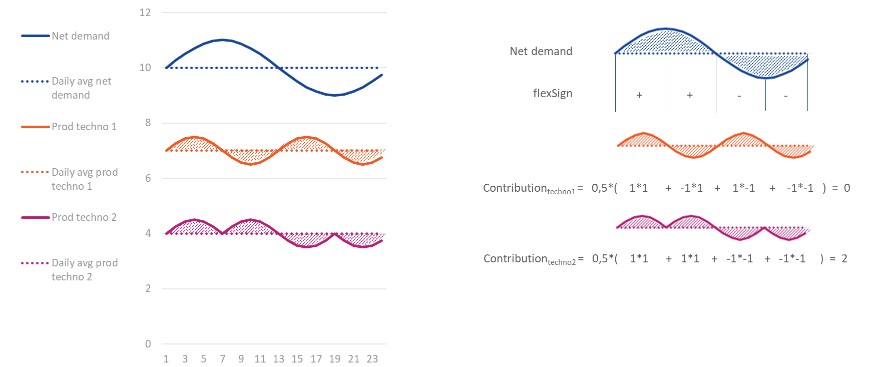
\[ \begin{align}\begin{aligned}flexibilityProdCurve_{techno}(t) = Prod_{techno}AtSubGranularity(t) - Prod_{techno}AvgAtFlexibilityGranularity(t)\\contribution_{techno} = \frac{1}{2} \sum_{\forall~time~steps~t} flexibilityProdCurve_{techno}(t) * flexSign(t)\end{aligned}\end{align} \]

Example of calculation of the contributions for daily flexibility needs for one day, with two technologies. Compared to the equations above, “net demand” is used instead of “residual load”.

For more information about the flexibility needs definition, please refer to Flexibility needs indicator

Curtailment cost (euro)¶

Indexed by

node
energy (electricity or gas)
technology
asset name
test case

The curtailement cost represents the cost, for the system, associated to curtailing or not using RES energy production. The KPI thus computes the total cost associated to the sum of annual volumes of Renewable Energy Sources (RES) production that is curtailed and annual volumes of RES production that is not used, per technology.

This cost is calculated by multplying the volume of RES production that is curtailed by the value for the system associated to this RES production, which, in the case of RES assets, is the difference between the incentives and the production cost.

The formula used is thus the following:

\[\small curtailmentCost_{RES techno} = \small \sum_t (installedCapa_{t}^{RES techno}*availability_{t}^{RES techno} - \small \sum_t prod_{t}^{RES techno})* \small RESproductionValue^{RES techno}\]

Where:

\[\small RESproductionValue_{RES techno} = incentive_{RES techno} - productionCost_{RES techno}\]

Results are given for electricity and gas production

Curtailment (Wh)¶

Indexed by

node
energy
technology
asset name
test case

Return the sum of annual volumes of production that is curtailed and annual volumes of production that is not used, per technology. It is calculated as the difference between the possible RES production (i.e. the installed capacity times the availability) and the actual RES production, per node, per technology:

\[\small curtailment_{techno} = \sum_{RES asset} (\sum_t installedCapacity_{t, asset}^{techno}*availability_{t, asset}^{RES asset} - \sum_t production_{t, asset}^{techno})\]

Demand peak (W)¶

Indexed by

node
energy
demand type
test case

Return the maximum value of the demand over the year, for a given node, energy, scenario and the demand asset type.

NB: In case of flexible demand, we here consider realized demand (after optimization)

Warning: Total of selected technologies corresponds for each (node, energy, test case) to a maximum over a sum of data. This calculation cannot be reproduced via aggregation.

Demand (Wh)¶

Indexed by

node
energy
demand type
asset name
test case

Return the annual volumes of energy demand for a given technology or contract. We here consider the flexible demand after optimization (using the consumption of the corresponding assets). This demand can be negative for asset “Voluntary load curtailment”. For asset “Electric Vehicles” with behavior Vehicule to grid, the demand is the difference between consumption and generation of the vehicles.

Detailed Demand (Wh)¶

Indexed by

zone
node
energy
sector
subsector
end use
equipment

Returns the annual volumes of energy demand according to the context’s demand graph.

Dispatchable power generation capacity (W)¶

Indexed by

node
energy (electricity, gas, hydrogen or heat)
technology
test case

Return the annual mean dispatchable capacity per node and technology, i.e. the mean capacity of assets that can be switched on at will (i.e. the mean capacity of assets other than “must-run” assets). The mean dispatchable capacity is calculated as the sum over the dispatchable assets, of the installed capacity times the mean availability:

\[\small meanDispatchCapa_{node} = \sum_{asset} installedCapa_{asset}^{node}*mean_t(availability_{t, asset})\]

Where \(\small meanDispatchCapa_{node}\) is the mean dispatchable capacity for a given node and \(\small installedCapa_{asset}^{node}\) is the installed capacity of a dispatchable asset.

Exports and imports (Wh)¶

Indexed by

node
energy (electricity, gas, hydrogen or heat)
test case
technology
asset name
data type (exports or imports)

Return the annual volumes of energy imported and exported by a given node.

Flexibility needs (Wh)¶

Indexed by

node
flexibility granularity (Daily, Weekly and Annual)
Test cases

Flexibility needs for power systems are calculated on the basis of the residual load and facilitate the understanding of the extent to which rising RES shares increase these needs. Responding to these needs would lead to a fully smoothened net load that could be fully satisfied by baseload capacities.

The residual load is computed by subtracting the renewable must-run generation from the demand. The above listed asset types are included in this must-run generation:

Solar : ‘Solar fleet’

Wind : ‘Wind onshore fleet’ and ‘Wind offshore fleet’

Hydro : ‘Hydro RoR fleet’ and the must-run generation part of ‘Hydro fleet’, i.e. \(\small \_minLoad \times \_pmax \times \_availability\)

FLEXIBILITY GRANULARITY

Daily flexibility needs are defined as the difference between the hourly residual load throughout a day and its daily average. The result is expressed as a volume of energy per day (e.g. GWh/day). Summing up these daily (positive) differences over the whole simulation (365 days for a single year simulation) reveals the overall daily flexibility needs one may respond to in order to obtain a residual load that is flattened out on a daily basis.

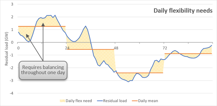
Daily flexibility needs definition

A similar calculation is realised in order to obtain the weekly flexibility needs, comparing the daily averages of the residual load (i.e. the residual load after having replied to all daily flexibility needs) with the mean residual load across each week. Summing up the weekly flexibility needs of all weeks gives the overall weekly flexibility needs.

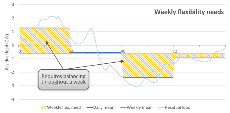
Weekly flexibility needs definition

Last, annual flexibility needs are determined as the cumulated difference between the monthly averages and the mean residual load across the entire year

EQUATIONS:

In the equations below, ResidualLoadAvgAtFlexibilityGranularity refers to the residualLoad average at the granularity of the indicator (weekly average for weekly granularity for example), and ResidualLoadAvgAtSubGranularity to the average at the subGranularity (daily average for weekly granularity).

In the figures above, “ResidualLoadAvgAtFlexibilityGranularity” corresponds to the red curve, and ResidualLoadAvgAtSubGranularity to the blue curve.

\[flexibilityCurve(t) = ResidualLoadAvgAtSubGranularity(t) - ResidualLoadAvgAtFlexibilityGranularity(t)\]

\[flexSign(t) = sign(flexibilityCurve(t))\]

\[\begin{split}\begin{eqnarray} flexibilityNeeds &=& \sum_{\forall~time~steps~t} flexibilityCurve^{+}(t) \\ &=& \frac{1}{2} \sum_{\forall~time~steps~t} \vert flexibilityCurve(t) \rvert \\ &=& \frac{1}{2} \sum_{\forall~time~steps~t} flexibilityCurve(t) * flexSign(t) \end{eqnarray} \end{split}\]

Flow (Wh)¶

Indexed by

energy (electricity, gas, hydrogen or heat)
test case
transmission

Return the annual volumes flowing through a considered transmission line (monodirectionnal).

Import capacity (W)¶

Indexed by

node
energy (electricity, gas, hydrogen or heat)
test case

This KPI will return No data on power contexts and gas contexts without import or export contracts as it only applies to gas import and export contracts.

Return the import capacity of a given node for a given energy and a given scenario.

Installed capacities (W)¶

Indexed by

node
energy (electricity, gas, hydrogen or heat)
technology
asset name
test case

Return the installed capacity of a given technology, for a given node and a given scenario combination.

Investment Analysis (euro)¶

Indexed by

energy
test case
production asset

The Investment Analysis calculates the economic profitability of a given production asset in a given node, defined as the difference between the producer surplus and the investment costs for this specific asset.

The producer surplus is calculated as the benefit the producer receives for selling its product on the market. The investment costs is the sum of the Capital Expenditure (CAPEX) and Fixed Operating Cost (FOC):

\[\small investmentAnalysis_{asset} = \small producerSurplus_{asset} - investmentCosts_{asset}\]

with:

\[\small investmentCosts_{asset} = \small \sum_t installedCapacity^{asset}*(CAPEX^{asset} + FOC^{asset})\]

and:

\[\small producerSurplus_{asset} = \small \sum_t (production_{t, asset}.marginalCost_{t, node, energy}) - productionCost_{asset}\]

Warning: in pathway optimization mode, this KPI may give incorrect values. Please launch the optimization with context parameter ‘Resimulate after capa optim’ at True to ensure that you get right marginal costs.

Investment costs (euro)¶

Indexed by

node
energy (electricity, gas, hydrogen or heat)
test case
technology
asset name

Return the investment costs per technology, i.e. the cost associated to building a given technology. It is equal to the technology installed capacity times the sum of the CAPEX and Fixed Operating Cost (FOC):

\[\small investmentCosts_{techno, energy} = installedCapacity^{techno, energy}*(CAPEX^{techno, energy} + FOC^{techno, energy})\]

Load payment (euro)¶

Indexed by

node
energy
test case

The load payment corresponds to the price consumers must pay for the energy consumed over the year, in a given node. It is calculated as the sum, over the year, of the hourly marginal cost of the node for the corresponding energy times the hourly demand for this energy in the node.

For a given energy, the load payment is computed as follows:

\[\small loadPayment_{node, energy} = \sum_t marginalCost_t^{node, energy}*demand_t^{node, energy}\]

Warning: in pathway optimization mode, this KPI may give incorrect values. Please launch the optimization with context parameter ‘Resimulate after capa optim’ at True to ensure that you get right marginal costs.

Loss of load cost (euro)¶

Indexed by

node
energy
test case

The loss of load cost is the cost associated to loss of load (LoL) in an energy system. In classic models, this cost is directly indexed on the value of loss of load (VoLL), which is the amount customers would be willing to pay in order to avoid a disruption in their electricity service. This leads to the following formulation:

\[\small LoLcost_{node} = \sum_t VoLL^{node}.LoL_t^{node}\]

Loss of load volume (Wh)¶

Indexed by

node
energy
test case

The Expected Unserved Energy is the annual volume of energy (including reserves) that is not served, i.e. the annual volume of a given energy that is needed but is not delivered due to a lack of generation.

Loss Of Load (h)¶

Indexed by

node
energy
test case

Loss Of Load (LOL), also called Loss Of Load Expectation (LOLE) represents the number of hours per year in which there is a situation of loss of load (i.e. that supply does not meet demand). It takes into account the fact that if the LOL is “too large”, then additional capacities (power plants or batteries) will be built.

\[\small LOL = \sum_t \mathbf 1_{\{supply_t < demand_t\}}\]

Marginal costs statistics (euro/MWh)¶

Indexed by

node
energy (electricity, reserve or gas)
test case
statistics (min, max, average or demand average)

Computes the minimum, maximum and average value of the marginal cost over the year for a given node and energy.

The KPI also computes the demand weighted (demand average) marginal cost:

\[\small demandWeightedMarginalCost_{node, energy} = \frac{\sum_t marginalCost_t^{node, energy}.demand_t^{node, energy}}{\sum_t demand_t^{node, energy}} \]

The marginal cost of a given energy and a given node is the variable cost of the production unit that was last called (after the costs of the different technologies were ordered in increasing order) to meet the energy demand in the node.

Warning: in pathway optimization mode, this KPI may give incorrect values. Please launch the optimization with context parameter ‘Resimulate after capa optim’ at True to ensure that you get right marginal costs.

Minimum unused production capacity (W)¶

Indexed by

node
energy
test case
technology

Minimal margin between available capacity and energy production for a given node, for a given energy and a given technology:

\[\small minMargin_{node, techno, energy} = \min_t availability_{t, node, techno, energy} \times pmax_{t, node, techno, energy} - production_{t, node, techno, energy}\]

Warning: Total of selected technologies corresponds for each (node, energy, test case) to a minimum over a sum of data. This calculation cannot be reproduced via aggregation.

Net demand peak (W)¶

Indexed by

node
energy (electricity, gas, hydrogen or heat)
test case

Return the maximum value over the year of the net demand, which is defined as the difference between the realized energy demand and the available capacity of flexible renewable energy at a given node:

\[\small netDemandPeak_{node} = max_t(demand_t^{node} - availableRenewableCapacity_t^{node})\]

Net Production (Wh)¶

Indexed by

node
energy
test case
technology
asset name

Return the total energy production in a given node, a given energy and a given technology minus the consumption on the same period.

\[\small production_{node, energy, techno} = \sum_t (production_{t, node, energy, techno} - consumption_{t, node, energy, techno})\]

Overnight investment costs (current euro/period)¶

Indexed by

node
energy (electricity, gas, hydrogen or heat)
test case
technology (Production, storage and transmission types)
asset name
type of cost (Capex, Deinvest or Repowering)
period
pathway

Unit: euro_current/period

The actualisation is not taken into account in this KPI (even if costs are actualized in the objective function). This means that a context in 2040 gives its results in euro_2040. Returns the overnight investment costs per technology, i.e. the cost associated to building a given technology. It includes the investment, the decommissioning and the repowering cost. The objective of this KPI is to identify the years when investments costs are highest. Investment and repowering costs include the premium, which captures the cost of financing an asset and the financial risk associated, and the ratio avoiding side effects if the lifetime of the asset expires after the end of the pathway horizon

\[\begin{split}\small overnightInvestmentCosts_{techno, energy, period} & = INVESTMENT_{COST}*(add-add_{repowering}) + DEINVEST_{COST}*(less-add_{repowering}) \\ & + REPOWERING_{COST}*add_{repowering}\end{split}\]

Pathway CO2 emissions (tCO2/pathway)¶

Indexed by

node
technology
asset name
test case

Unit: tCO2/pathway

This KPI represents the total volume of CO2 emissions emitted during the entire pathway. The emissions taken into account are those due to energy production (energy + reserve). It is calculated as the sum over the hours of the whole pathway, of the CO2 emissions/MWh multiplied by the volume of produced energy for each asset:

\[\small pathwayCo2Emissions_{scenario} = \sum_{pathwayStep} duration_{pathwayStep} \sum_{node} \sum_{technology} \sum_{t} CO2perMWh*producedEnergy_{pathwayStep, node, techno, t, scenario}\]

CO2 emissions due the reserve activation (balancing) are not calculated by this KPI.

Pathway total costs (constant euro of the first pathway year/pathway)¶

Indexed by:

node
types of possible scenarios
energy
technology
type of cost

Unit: euro_constant_first_pathway_step

The actualisation is taken into account in this KPI (even if costs are actualized in the objective function). For each period of the pathway, this KPI computes the total cost associated (see KPI Total Costs) and multiply it by the actualization ratio. Returns the total costs associated to a pathway for :

satisfying the demand (power and reserve)

investing in new capacities (production, transmission and storage)

for a given node and pathway for each scenario :: \[\begin{split}\small pathwayTotalCosts_{node} & = \sum_{pathwaySteps} ( \small investmentCost_{node, pathwayStep} + \small variableOperatingCost_{node, pathwayStep} \\ & + \small fixedOperatingCost_{node, pathwayStep} ) * yearWeight_{pathwayStep}\end{split}\]
with: \[\begin{split}\small investmentCosts & = \small annualizedInvestmentCost_{optimized assets} + \small annualizedInvestmentCost_{unoptimized assets} + \small decommissioningCost_{optimized assets} \\ & + \small repoweringCost_{optimized assets}\end{split}\]

\[\small variableOperatingCosts = \small productionCost + \small co2Cost + \small fuelCost + \small transmissionCost + \small storageCost + \small lossOfLoadCost\]

\[\small yearWeight = \small initialWeight * (\frac{1}{1+R})^{\small pathwayStepYear - \small firstYearOfPathway}\]

Producer surplus (euro)¶

Indexed by

reference node
test case
technology
asset name

A producer surplus occurs when the producer is paid more for a given product than the minimum amount it is willing to pay for its production. It represents the benefit the producer receives for selling its product on the market.

The KPI thus computes the difference between the amount an energy producer receives and the minimum amount the producer is paying for the energy it produces, i.e. the production times the marginal cost (the amount the producer receives) minus the production cost and the marginal consumption cost if there is one (the amount the producer has paying). And to compute the producer revenue, we need to consider all its “primary energy productions” and consumptions (electricity, reserve energies,…), but not the secondary ones (fuel, co2,…).

For each scenario \(s\), node \(n\) and technology \(T\) :

\[\begin{split}\small productionSurplusKpi_{s, n, T} = \small \sum_{asset\ a\ |\ refNode(a)==n\ \\and\ technology(a)==T} ( \sum_{time\ step\ t} (\sum_{primary\ produced\ \\energy\ e\ of\ a} production_{ct s, t, a, e} \times margCost_{s, t, e, prodNode(a,e)} - \sum_{primary\ consumed\ \\energy\ e'\ of\ a} consumption_{s, t, a, e'} \times margCost_{s, t, e', consumptionNode(a,e')}) \\ \small - productionCost_{s, a})\end{split}\]

Where \(\small productionCost_{s, a}\) is the total production cost of the asset for a given scenario (cf the “Production costs” KPI documentation).

Production costs (euro)¶

Indexed by

reference node
test case
technology
asset name

The KPI computes the total production costs in a given node and a given technology.

So for each scenario \(s\), asset \(a\) and time step \(t\), asset costs fall in the various categories below :

\[\small variableCost_{s, t, a} = production_{s, t, a, mainEnergy} \times (productionCost_{s, t, a} \times \delta_{notActive(BH\_CLUSTER)} + variableCost_{s, t, a} \times \delta_{isActive(BH\_CLUSTER)})\]

\[\small runningCapacityCost_{s, t, a} = runningCapacityCost_{s, t, a} \times runningBound_{s, t, a}\]

\[\small startUpCost_{s, t, a} = startUpIndexedCost_{s, t, a} \times startingCapacity_{s, t, a}\]

\[\small fuelCost_{s, t, a} = \small \sum_{fuelEnergy} fuelConsumption_{s, t, a, fuelEnergy} \times marginalCost_{s, t, fuelEnergy, fuelNode(fuelEnergy, a)}\]

where \(\small fuelNode(fuelEnergy, a)\) is the node where the asset \(a\) consumes the fuel energy \(\small fuelEnergy\)

\[\small consumptionCost_{s, t, a} = consumption_{s, t, a, mainEnergy} \times consumptionIndexedCost_{s, t, a}\]

\[\small co2EmissionsCost_{s, t, a} = co2Emissions_{s, t, a, co2Energy} \times marginalCost_{s, t, co2Energy, co2Node(co2Energy,a)}\]

where \(\small co2Node(co2Energy,a)\) is the node where the asset \(a\) produces the fuel energy \(\small co2Energy\)

\[\small storageCost_{s, t, a} = storageLevel_{s, t, a} \times storageLevelIndexedCost_{s, t, a}\]

For each reserve energy :

\[\small reserveCost_{s, t, a, reserveEnergy} = production_{s, t, a, reserveEnergy, RUNNING} \times reserveProdCost_{s, t, a, reserveEnergy}\]

\[\small reserveNotRunningCost_{s, t, a} = production_{s, t, a, mfrrUp, NOT\_RUNNING} \times notRunningReserveCost_{s, t, a, mfrrUp}\]

So we can define the total production cost of an asset as :

\[\small productionCost_{s, a} = \sum_t variableCost_{s, t, a} + runningCapacityCost_{s, t, a} + startUpCost_{s, t, a} + fuelCost_{s, t, a} + consumptionCost_{s, t, a} + co2EmissionsCost_{s, t, a} + storageCost_{s, t, a}\]

\[\small + \sum_{reserveEnergy} reserveCost_{s, t, a, reserveEnergy} + reserveNotRunningCost_{s, t, a}\]

NB : All costs of a given asset must always be considered together, since some costs are shared. For instance, the runningCapacityCost is linked to the electricity production as much as to the reserve production. Therefore, indexing these costs by energy would be misleading. It is also true for the indexing by node : an asset could produce or consume at several nodes, but divide its cost on several nodes would be misleading and wrong. For practicality purposes, we just index this KPI by reference node, each asset having a single reference node (classically the node where the asset produces its main energy production).

So for each scenario \(s\), node \(n\) and technology \(T\), we have :

\[\begin{split}\small productionCostKpi_{s, n, T} = \sum_{time\ step\ t} \sum_{asset\ a\ |\ refNode(a)==n\ \\and\ technology(a)==T} productionCost_{s, a}\end{split}\]

Production revenue (euro)¶

Indexed by

node
energy
test case
technology
asset name

Return the annual revenue received by a given technology in a given node, for the energy it produces.

It is calculated as the sum over the year of the production of the technology times the marginal cost within the considered node:

\[\small revenue_{techno, node} = \sum_t production_t^{techno, node}.marginalCost_t^{node}\]

Production (Wh)¶

Indexed by

node
energy
test case
technology
asset name

Total energy production in a given node, for a given energy and a given technology:

\[\small production_{node, techno, energy} = \sum_t production_{t, node, techno, energy}\]

Raw demand (Wh)¶

Indexed by

node
energy
demand type
test case

Return the annual volumes of unoptimized energy demand for a given technology or contract. We consider here the flexible demand before optimization (using the objective demand of the corresponding assets).

This demand will be 0 for asset “Voluntary load curtailment” since it is price activated and as no consumption objectives. For asset “Electric Vehicles” with behavior Vehicule to grid, this demand does not consider any production, since V2G is price activated too.

Scarcity Price Hours (h)¶

Indexed by

node
energy
test case

Return the number of hours where marginal costs of a node is higher than a certain value reflecting scarcity of production capacity at said hours.

Warning: in pathway optimization mode, this KPI may give incorrect values. Please launch the optimization with context parameter ‘Resimulate after capa optim’ at True to ensure that you get right marginal costs.

Storage capacity (Wh)¶

Indexed by

node
energy (electricity, gas, hydrogen or heat)
technology
asset name
test case

Return the storage capacity per node, per energy and technology (in Wh).

Storage costs (euro)¶

Indexed by

energy
storage asset
test case

Storage cycles (cycles)¶

Indexed by

node
energy (electricity, gas, hydrogen or heat)
test case

For a given node, computes the equivalent number of full discharge cycles of all the cycling storage units within the node, based on their annual production and their production capacity.

Storage surplus (euro)¶

Indexed by

energy
storage asset
test case

The storage surplus is the benefit made when storing energy instead of using it directly.

Warning: in pathway optimization mode, this KPI may give incorrect values. Please launch the optimization with context parameter ‘Resimulate after capa optim’ at True to ensure that you get right marginal costs.

Supply-demand balance (Wh)¶

Indexed by

node
energy
test case
technology
asset name
data type (Supply and Demand)

Returns the annual volumes of energy demand and supply for every energy, node, asset and technology of a given context

Supply (Wh)¶

Indexed by

node
energy (any energy, fuel and reserve type)
test case
technology
asset name

Return for a given node, the annual volumes of production per technology, as well as the imports to the node through the transmissions and the fuel supply. It is similar to the KPI ‘Production’ but it also includes imports and fuel supply.

The KPI is particularly adapted for gas models as national gas demand is in large parts satisfied by imports.

Total costs (current euro/period)¶

Indexed by:

node
test case
energy
technology
asset name
type of cost

Unit: euro_current/period

The actualisation is not taken into account in this KPI (even if costs are actualized in the objective function). This means that a context in 2040 gives its results in euro_2040. The cost is given per period. This means that for a ten year duration period, you have to multiply the displayed cost by 10 to get the total cost over the period. Returns the sum of the investment, variable operating and fixed operating costs of all the assets. These costs are annualized and distributed over the lifetime of the assets they are attached to. Investment and repowering costs include the premium, which captures the cost of financing an asset and the financial risk associated, and the ratio avoiding side effects if the lifetime of the asset expires after the end of the pathway horizon.

\[\small totalCosts_{node, scenario} = \small investmentCost_{node, scenario} + \small variableOperatingCost_{node, scenario} + \small fixedOperatingCost_{node, scenario} \]

with: \[\begin{split}\small investmentCosts & = \small annualizedInvestmentCost_{optimized assets} + \small annualizedInvestmentCost_{unoptimized assets} + \small decommissioningCost_{optimized assets} \\ & + \small repoweringCost_{optimized assets}\end{split}\]

\[\small variableCosts = \small productionCost + \small co2Cost + \small fuelCost + \small transmissionCost + \small storageCost + \small lossOfLoadCost\]

Transmission capacities (W)¶

Indexed by

node
energy (electricity, gas, hydrogen or heat)
test case
transmission

Return the capacity of each single transmission. No data is returned if behavior Flow-Based is activated.

Transmissions costs (euro)¶

Indexed by

energy
transmission line
test case

Transmission usage (%)¶

Indexed by

node (dummy)
energy
test case
transmission

The instant transmission usage of an interconnection is the ratio of electricity or gas flowing through the transmission over its capacity. The KPI computes the yearly average value of instant transmission usage, for a given transmission:

\[transmissionUsage_{transmission} = \small \frac{mean_{t}(instantTransmissionUsage_{t}^{transmission})}{installedCapacity^{transmission}} (\%)\]

No data is returned if behavior Flow-Based is activated.

Variable operating costs (euro)¶

Indexed by:

node
types of possible scenarios

Return the total costs associated to satisfying the demand (for electricity and reserve), for a given node and context type, as the sum of the production costs, the loss of load costs, the loss of reserve costs and the curtailment costs:

\[\begin{split}\small totalCosts_{node} & = \small productionCost_t^{node} + \small lossOfLoadCost^{node} \\ & + \small lossOfReserveCost^{node} + \small CurtailmentCost^{node} \end{split}\]

Variation in installed CCUS capacities (t/h/year)¶

Indexed by

node
energy (co2_captured)
technology
asset name
test case
type of change (add or less)

Unit: t/h/year

The variations in capacity are given per year. This means that for a ten year duration period, you have to multiply the displayed value by 10 to get the total variation in capacity over the period. This represents the yearly average variations in installed capacities during the period which just ended. For example add_2030 gives the capacity added during the period ending in 2030. By definition, add and less values are 0 for the first period. Returns the variations in installed capacity of a given technology for assets optimized at least during one period in the pathway, for a given node and a given scenario combination.

Variation in installed capacities (W/period)¶

Indexed by

node
energy (electricity, gas, hydrogen or heat)
technology
asset name
test case
type of change (add or less)

Unit: W/period

The variations in capacity are given per period. This represents the overall variation in installed capacities during the period which just ended. For example add_2030 gives the capacity added during the period ending in 2030. By definition, add and less values are 0 for the first period. Returns the variations in installed capacity of a given technology for assets optimized at least during one period in the pathway, for a given node and a given scenario combination.

Welfare (euro)¶

Indexed by

node
test case

The welfare for a given node is the sum of its consumer surplus, its producer surplus, the border exchange surplus and half of the congestion rent for power transmission lines connected to the node:

\[\small welfare_{node, tc} = consumerSurplus_{node, tc} + producerSurplus_{node, tc} + exchangeSurplus_{node, tc} + \frac{1}{2} \sum_{transmission\ t \in node} congestionRent_{t, tc}\]

Warning: in pathway optimization mode, this KPI may give incorrect values. Please launch the optimization with context parameter ‘Resimulate after capa optim’ at True to ensure that you get right marginal costs.

All results¶

Indexed by

node
energy
technology
asset
result type
test case

This view shows the time series of the basic, unprocessed results associated with the assets and nodes selected. The following results are covered:

Energy production for assets

Energy consumption for assets

Production (or variable) costs for assets

Marginal costs for nodes

Storage level for assets

Startup costs for assets

Running costs for assets

Running bound for assets

Running stock for assets

Warning: in pathway optimization mode, this KPI may give incorrect values. Please launch the optimization with context parameter ‘Resimulate after capa optim’ at True to ensure that you get right marginal costs.

Consumption vs production view (W)¶

Indexed by

asset
data
test case

This view shows a time series of the electricity production and consumption of the selected asset, as well as the running capacity.

Contract view (W)¶

Indexed by

asset
test case

This view shows the result of the financial asset, as a time series

Cumulative demand (Wh)¶

This view shows, for each energy, a temporal cumulative view showing how the energy demand is divided by technology at this node. The demands are here shown after optimization (using the consumption of the corresponding assets). This demand can be negative for asset “Voluntary load curtailment”. For asset “Electric Vehicles” with behavior Vehicule to grid, the demand is the difference between consumption and generation of the vehicles.

Cumulative generation (W)¶

This view shows a temporal cumulative view, for each energy, of the generation at the selected node for each generation technology at every time step as well at the demand level.

Demand and Net Demand (W)¶

This view shows time series, for each energy, of the demand and net demand, both optimized and unoptimized, for this energy at the selected node. Unoptimized net demand is defined as the difference between unoptimized demand and the must run available capacity. Optimized net demand is defined as the difference between optimized demand and the must run generation.

Electricity CO2 content (t/MWh)¶

indexed by:

node
energy
context
test case

Returns produced and consumed electricity co2 contents timeseries for each node. It accounts for the physical flows of CO2 and therefore does not take into account the cancellation of the carbon footprint of biogas or biomass fueled plants.

To compute the consumed electricity CO2 content, we rely on the proportional sharing hypothesis, which states that at every node, the output of each asset is distributed according to the value of the flows. It allows to write a balance of supply and demand for each asset :

\[\begin{split}&G_{\alpha}^n + \sum_{m} q_{\alpha}^m F_{m,n} = q_{\alpha}^n P_n \\ \Leftrightarrow &G_{\alpha}^n = \sum_{m} q_{\alpha}^m(\delta_{m,n}P_m - F_{m,n})\end{split}\]

with :

\(G_{\alpha}^n\): Production of asset \(\alpha\) (including stock) at node \(n\), and \(G_{\alpha}\) is the associated column vector (which therefore only has one non-zero row corresponding to the node to which \(\alpha\) is connected).
\(q_{\alpha}^n\): The portion of electricity consumed at node \(n\) produced by asset \(\alpha\) (in [0,1]), and \(q_{\alpha}\) is the associated column vector.
\(P^n\): The nodal load at node \(n\) (production + imports = consumption + exports)
\(F_{i,j}\): Transmission flow between nodes i and j, with \(F_{i,i}=0\) by convention.

This can be rewritten as :

\[\forall (n,\alpha), \sum_{m} \left(\delta_{m,n} - \frac{F_{m,n}}{P_m}\right) P_m q^m_{\alpha} = G_{n,\alpha}\]

Which represents for every technology \(\alpha\) a NxN system which can be rewritten in matrix form, with matrix \(D\) such that \(D_{n,m}=\frac{F_{m,n}}{P_m}\) :

\[(I-D)\text{diag}(P)q_{\alpha} = G_{\alpha}\]

We thus can find the proportion of electricity consumed at each node produced by each technology \(q_{\alpha}^n\) by inverting:

\[q_{\alpha} = [(I-D)\text{diag}(P)]^{-1} G_{\alpha}\]

Finally the consumed electricity co2 content can be computed as the weighted average of the production carbon contents of assets \(\alpha\) by their participations \(q_{\alpha}^n\).

\[x_n = \sum_{\alpha} \text{CO2content}_{\alpha} q_{\alpha}^n = \sum_{\alpha} \text{CO2content}_{\alpha} [AG_{\alpha}]^n\]

Let \(E\) be the vector of CO2 emissions (total emissions by country in t CO2): \(E = \sum_{\alpha} \text{CO2content}_{\alpha} G_{\alpha}\)

The column vector \(X\) of the CO2 contents of electricity consumed by node is obtained:

\[X = A \cdot E = [(I - D)\text{diag}(P)]^{-1} E\]

Consumption view (Fuel) (W)¶

Indexed by

asset
data
test case

This view shows the fuel consumption of the asset, in W. It considers whether fleet mode and cluster mode, and displays the appropriate results.

Stacks:

(Cluster mode only) Fuel consumption from energy making
(Cluster mode only) Fuel consumption from running capacity

Lines:

Fuel consumption
Absolute minimal fuel consumption (0 in cluster mode, as the running capaciy has no lower boundary)
Absolute maximal fuel consumption calculated from installed capacity
Absolute maximal fuel consumption calculated from available capacity

Consumption view (Gas) (W)¶

Indexed by

asset
data
test case

This view shows a time series of the gas consumption of the asset.

Production view (Gas) (W)¶

Indexed by

asset
data
test case

This view shows a time series of the gas production of the asset as well as levels of minimal generation and available capacity.

Marginal costs (euro/MWh)¶

This view shows a time series, for each energy, of the marginal cost of generation of this energy at the selected node.

Warning: in pathway optimization mode, this KPI may give incorrect values. Please launch the optimization with context parameter ‘Resimulate after capa optim’ at True to ensure that you get right marginal costs.

Net Position (Wh)¶

Indexed by

node
energy
time
test case

This view shows a time series of the hourly balanced volume of energy (volume of energy exported minus the hourly volume of energy imported), for a selected node.

Production cost view (euro)¶

Indexed by

asset
data
test case

This view shows the time series of the production cost of the selected asset, as a stacked chart that cumulates the following costs:

CO2 emission cost
Consumption cost
Fuel consumption cost
MFFR downward reserve cost
MFFR up not running cost
MFFR upward reserve cost
Production cost
Running cost
Start up cost
Storage cost
Synchronized downward reserve cost
Synchronized upward reserve cost

Warning: in pathway optimization mode, this KPI may give incorrect values. Please launch the optimization with context parameter ‘Resimulate after capa optim’ at True to ensure that you get right marginal costs.

Production margin (W)¶

Margin at each time step between available capacity and energy production for a given delivery point, for a given energy and a given technology:

\[\small minMargin_{t, node, techno, energy} = availability_{t, node, techno, energy} \times pmax_{t, node, techno, energy} - production_{t, node, techno, energy}\]

Production view (W)¶

Indexed by

asset
data
test case

This view shows a combination of time series as stacks and lines.

Stacks:

Non reserved generation
Downward MFRR
Downward Synchronized Reserve
Upward Synchronized Reserve
Upward MFRR

Lines:

Generation capacity
Available capacity
Running Bound
Generation level
Minimal Generation level

Stocks (Wh)¶

This view shows, for each energy, a pie chart showing how the storage capacity is divided by technology.

Storage view (Wh)¶

Indexed by

asset
data
test case

This view shows a combination of time series as stacks and lines.

Stacks:

Production
Fixed demand
Consumption
Fixed supply
Bounded supply (includes Prorata supply)

Lines:

Maximum storage capacity
Available storage capacity
Storage level
Minimal storage level

Transmission consumption view (W)¶

Indexed by

asset
data
test case

This view shows a time series of the consumption of the selected transmission asset as well as the available consumption capacity. Note that the available consumption capacity is only returned when the flow-based behavior is not activated.

Transmission production view (W)¶

Indexed by

asset
data
test case

This view shows a time series of the generation of the selected transmission asset as well as the available production capacity. Note that the available production capacity is only returned when the flow-based behavior is not activated.

KPI documentation¶

Average production at peak demand (W)¶

Border exchange surplus (euro)¶

Capacity factor (%)¶

Carbon sequestration (t)¶

CCUS installed capacities (t/h)¶

Carbon capture, usage and storage (t)¶

CO2 emissions (t)¶

Congestion hours (h)¶

Congestion Rent (euro)¶

Consumer Surplus (euro)¶

Consumption peak (W)¶

Consumption (Wh)¶

Contribution to flexibility needs (Wh)¶

Curtailment cost (euro)¶

Curtailment (Wh)¶

Demand peak (W)¶

Demand (Wh)¶

Detailed Demand (Wh)¶

Dispatchable power generation capacity (W)¶

Exports and imports (Wh)¶

Flexibility needs (Wh)¶

Flow (Wh)¶

Import capacity (W)¶

Installed capacities (W)¶

Investment Analysis (euro)¶

Investment costs (euro)¶

Load payment (euro)¶

Loss of load cost (euro)¶

Loss of load share (% of demand)¶

Loss of load volume (Wh)¶

Loss Of Load (h)¶

Marginal costs statistics (euro/MWh)¶

Minimum unused production capacity (W)¶

Net demand peak (W)¶

Net Production (Wh)¶

Overnight investment costs (current euro/period)¶

Pathway CO2 emissions (tCO2/pathway)¶

Pathway total costs (constant euro of the first pathway year/pathway)¶

Producer surplus (euro)¶

Production costs (euro)¶

Production revenue (euro)¶

Production (Wh)¶

Raw demand (Wh)¶

Scarcity Price Hours (h)¶

Share of production in national demand (%)¶

Storage capacity (Wh)¶

Storage costs (euro)¶

Storage cycles (cycles)¶

Storage surplus (euro)¶

Supply-demand balance (Wh)¶

Supply (Wh)¶

Total costs (current euro/period)¶

Transmission capacities (W)¶

Transmissions costs (euro)¶

Transmission usage (%)¶

Variable operating costs (euro)¶

Variation in installed CCUS capacities (t/h/year)¶

Variation in installed capacities (W/period)¶

Welfare (euro)¶

All results¶

Consumption vs production view (W)¶

Contract view (W)¶

Cumulative demand (Wh)¶

Cumulative generation (W)¶

Demand and Net Demand (W)¶

Electricity CO2 content (t/MWh)¶

Consumption view (Fuel) (W)¶

Consumption view (Gas) (W)¶

Production view (Gas) (W)¶

Marginal costs (euro/MWh)¶

Net Position (Wh)¶

Production cost view (euro)¶

Production margin (W)¶

Production view (W)¶

Stocks (Wh)¶

Storage view (Wh)¶

Transmission consumption view (W)¶

Transmission production view (W)¶