Knitro / MATLAB reference
The interfaces used to call Knitro from the MATLAB environment mimic both the “solver-based” and “problem-based” approaches offered by MATLAB. The solver-based interface provides the following specialized function calls for various optimization model types:
knitro_lp for solving linear programs (LPs);
knitro_milp for solving mixed-integer linear programs (MILPs);
knitro_minlp for solving mixed-integer nonlinear optimization models (MINLPs);
knitro_nlneqs for solving nonlinear systems of equations;
knitro_nlnlsq for solving nonlinear least-squares models;
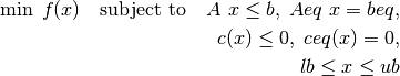
knitro_nlp for solving continuous nonlinear optimization models (NLPs);
knitro_qcqp for solving quadratically constrained quadratic programs (QCQPs) (this function can also be used to solve second order cone programs (SOCPs) by formulating the cone constraints as quadratic constraints);
knitro_qp for solving quadratic programs (QPs).
The Knitro/MATLAB interface also provides a generic knitro_solve function that can be used to solve any model defined using the problem-based approach.
In addition, the knitro_options function can be used to specify Knitro solver options for any of the above functions.
The Knitro/MATLAB interface functions are described in more detail below in alphabetical order.
Several examples using both the solver-based approach and problem-based approach are included in
the knitromatlab/examples directory provided with the Knitro distribution.
knitro_lp
Solve linear programs expressed in the form:

[x,fval,exitflag,output,lambda] = ...
    knitro_lp(f,A,b,Aeq,beq,lb,ub,x0,extendedFeatures,options,knitroOptsFile)
Input Arguments
f: Linear objective coefficients.
A: Coefficient matrix for linear inequality constraints.
b: Upper bound vector for linear inequality constraints.
Aeq: Coefficient matrix for linear equality constraints (optional).
beq: Right-hand side vector for linear equality constraints (optional).
lb: Variable lower bound vector (optional).
ub: Variable upper bound vector (optional).
x0: Initial point vector (optional).
extendedFeatures: Structure used to input additional model features, see The extendedFeatures Structure (optional).
options: Knitro options structure generated from knitro_options, see knitro_options (optional),
knitroOptsFile: Knitro options filename used to set Knitro options specified in a text file, see Setting options (optional).
Only the first three arguments are required. An empty argument can be specified using [].
Output Arguments
x: The optimal solution vector.
fval: The optimal solution objective value.
exitflag: Integer identifying the reason for termination of the algorithm.
output: Structure containing solution information about the optimization.
lambda: Structure containing the Lagrange multipliers at the solution with a different field for each constraint type.
Only the first output argument is required. An empty argument can be specified using [].
knitro_milp
Solve mixed-integer linear programs expressed in the form:
where x is composed of potentially both integer and continuous components as defined by the xType input array.
[x,fval,exitflag,output,lambda] = ...
    knitro_milp(f,xType,A,b,Aeq,beq,lb,ub,x0,extendedFeatures,options,knitroOptsFile)
Input Arguments
f: Linear objective coefficients.
xType: Specifies the variable type (should have the same dimension as x): 0 for continuous, 1 for general integer, and 2 for binary (set lb[i]=0 and ub[i]=1 for any binary variables). If xType=[], variables are assumed to be continuous.
A: Coefficient matrix for linear inequality constraints.
b: Upper bound vector for linear inequality constraints.
Aeq: Coefficient matrix for linear equality constraints (optional).
beq: Right-hand side vector for linear equality constraints (optional).
lb: Variable lower bound vector (optional).
ub: Variable upper bound vector (optional).
x0: Initial point vector (optional).
extendedFeatures: Structure used to input additional model features, see The extendedFeatures Structure (optional).
options: Knitro options structure generated from knitro_options, see knitro_options (optional),
knitroOptsFile: Knitro options filename used to set Knitro options specified in a text file, see Setting options (optional).
Only the first four arguments are required. An empty argument can be specified using [].
Output Arguments
x: The optimal solution vector.
fval: The optimal solution objective value.
exitflag: Integer identifying the reason for termination of the algorithm.
output: Structure containing solution information about the optimization.
lambda: Structure containing the Lagrange multipliers at the solution with a different field for each constraint type.
Only the first output argument is required. An empty argument can be specified using [].
knitro_minlp
Solve mixed-integer nonlinear optimization models expressed in the form:
where x is composed of potentially both integer and continuous components as defined by the xType input array.
[x,fval,exitflag,output,lambda,grad,hessian] = ...
    knitro_minlp(fun,x0,xType,A,b,Aeq,beq,lb,ub,nonlcon,extendedFeatures,options,knitroOptsFile)
Input Arguments
fun: The function to be minimized. fun accepts a vector x and returns a scalar f, the objective function evaluated at x. If exact/user-supplied gradients are used, an additional vector with the objective gradient should be returned.
x0: Initial point vector.
xType: Specifies the variable type (should have the same dimension as x): 0 for continuous, 1 for general integer, and 2 for binary (set lb[i]=0 and ub[i]=1 for any binary variables). If xType=[], variables are assumed to be continuous.
A: Coefficient matrix for linear inequality constraints.
b: Upper bound vector for linear inequality constraints.
Aeq: Coefficient matrix for linear equality constraints (optional).
beq: Right-hand side vector for linear equality constraints (optional).
lb: Variable lower bound vector (optional).
ub: Variable upper bound vector (optional).
nonlcon: The function that computes the nonlinear inequality and equality constraints. nonlcon accepts a vector x and returns two vectors: the values of the nonlinear inequality constraints at x and the values of the nonlinear equality constraints at x. If exact/user-supplied gradients are used, two additional matrices should be returned with the gradients for the nonlinear inequality constraints and the gradients for the nonlinear equality constraints (optional).
extendedFeatures: Structure used to input additional model features, see The extendedFeatures Structure (optional).
options: Knitro options structure generated from knitro_options, see knitro_options (optional),
knitroOptsFile: Knitro options filename used to set Knitro options specified in a text file, see Setting options (optional).
Only the first two arguments are required. An empty argument can be specified using [].
Output Arguments
x: The optimal solution vector.
fval: The optimal solution objective value.
exitflag: Integer identifying the reason for termination of the algorithm.
output: Structure containing solution information about the optimization.
lambda: Structure containing the Lagrange multipliers at the solution with a different field for each constraint type.
grad: Objective gradient vector at x.
hessian: Hessian matrix at x, lambda. For notes on when this option is available, see
KN_get_hessian_values().
Only the first output argument is required. An empty argument can be specified using [].
knitro_nlneqs
Solve square, nonlinear systems of equations:

[x,fval,exitflag,output,jacobian] = ...
    knitro_nlneqs(fun,x0,extendedFeatures,options,knitroOptsFile)
Input Arguments
fun: The functions whose components are to be solved to equal zero. fun accepts a vector x and returns a vector F, the values of the nonlinear equations evaluated at x. If exact/user-supplied gradients are used, an additional matrix should be returned with the Jacobian of the nonlinear equations at x. Unlike the user-supplied Jacobian for knitro_nlp/knitro_minlp, the entries J(i,j) of the Jacobian for knitro_nlneqs represent the partial derivative of the function component i with respect to variable j.
x0: Initial point vector.
extendedFeatures: Structure used to input additional model features, see The extendedFeatures Structure (optional).
options: Knitro options structure generated from knitro_options, see knitro_options (optional),
knitroOptsFile: Knitro options filename used to set Knitro options specified in a text file, see Setting options (optional).
Only the first two arguments are required. An empty argument can be specified using [].
Output Arguments
x: The optimal solution vector.
fval: The optimal solution objective value.
exitflag: Integer identifying the reason for termination of the algorithm.
output: Structure containing solution information about the optimization.
jacobian: The Jacobian matrix at x.
Only the first output argument is required. An empty argument can be specified using [].
knitro_nlnlsq
Solve a nonlinear least-squares model subject to bounds on the variables:

[x,resnorm,residual,exitflag,output,lambda,jacobian] = ...
    knitro_nlnlsq(fun,x0,lb,ub,extendedFeatures,options,knitroOptsFile)
Input Arguments
fun: The functions whose sum of squares is minimized. fun accepts a vector x and returns a vector F, the values of the functions/residuals evaluated at x. If exact/user-supplied gradients are used, an additional matrix should be returned with the Jacobian of the functions at x. Unlike the user-supplied Jacobian for knitro_nlp/knitro_minlp, the entries J(i,j) of the Jacobian for knitro_nlnlsq represent the partial derivative of the function component i with respect to variable j.
x0: Initial point vector.
lb: Variable lower bound vector (optional).
ub: Variable upper bound vector (optional).
extendedFeatures: Structure used to input additional model features, see The extendedFeatures Structure (optional).
options: Knitro options structure generated from knitro_options, see knitro_options (optional),
knitroOptsFile: Knitro options filename used to set Knitro options specified in a text file, see Setting options (optional).
Only the first two arguments are required. An empty argument can be specified using [].
Output Arguments
x: The optimal solution vector.
resnorm: The norm of the residuals at the solution.
residual: The vector of residuals at the solution.
exitflag: Integer identifying the reason for termination of the algorithm.
output: Structure containing solution information about the optimization.
lambda: Structure containing the Lagrange multipliers at the solution with a different field for each constraint type.
jacobian: The Jacobian matrix at x.
Only the first output argument is required. An empty argument can be specified using [].
knitro_nlp
Solve continuous nonlinear optimizaton models expressed in the form:
[x,fval,exitflag,output,lambda,grad,hessian] = ...
    knitro_nlp(fun,x0,A,b,Aeq,beq,lb,ub,nonlcon,extendedFeatures,options,knitroOptsFile)
Input Arguments
fun: The function to be minimized. fun accepts a vector x and returns a scalar f, the objective function evaluated at x. If exact/user-supplied gradients are used, an additional vector with the objective gradient should be returned.
x0: Initial point vector.
A: Coefficient matrix for linear inequality constraints.
b: Upper bound vector for linear inequality constraints.
Aeq: Coefficient matrix for linear equality constraints (optional).
beq: Right-hand side vector for linear equality constraints (optional).
lb: Variable lower bound vector (optional).
ub: Variable upper bound vector (optional).
nonlcon: The function that computes the nonlinear inequality and equality constraints. nonlcon accepts a vector x and returns two vectors: the values of the nonlinear inequality constraints at x and the values of the nonlinear equality constraints at x. If exact/user-supplied gradients are used, two additional matrices should be returned with the gradients for the nonlinear inequality constraints and the gradients for the nonlinear equality constraints (optional).
extendedFeatures: Structure used to input additional model features, see The extendedFeatures Structure (optional).
options: Knitro options structure generated from knitro_options, see knitro_options (optional),
knitroOptsFile: Knitro options filename used to set Knitro options specified in a text file, see Setting options (optional).
Only the first two arguments are required. An empty argument can be specified using [].
Output Arguments
x: The optimal solution vector.
fval: The optimal solution objective value.
exitflag: Integer identifying the reason for termination of the algorithm.
output: Structure containing solution information about the optimization.
lambda: Structure containing the Lagrange multipliers at the solution with a different field for each constraint type.
grad: Objective gradient vector at x.
hessian: Hessian matrix at x, lambda. For notes on when this option is available, see
KN_get_hessian_values().
Only the first output argument is required. An empty argument can be specified using [].
knitro_options
This function can be used to set Knitro user options (see Knitro user options).
options = knitro_options('optionname1',optionvalue1,'optionname2',optionvalue2,...)
options = knitro_options(oldoptions,'optionname1',optionvalue1,'optionname2',optionvalue2,...)
knitro_options returns an options structure generated from the input option/value pairs. The option names should be Knitro-specific option names (with the exception of UseParallel) input as strings and the values should only be numerical values (except UseParallel whose value should be true or false). The UseParallel option is a MATLAB-specific option that is recognized by knitro_options and can be used to implement parallel finite-difference evaluations through the Knitro/MATLAB interface.
If no arguments are provided, knitro_options returns all default option values. If the first parameter is an options structure then any additional option/value settings modify the passed in options structure. After generating an options structure using knitro_options, this structure can be passed to one of the Artelys Knitro (R) solvers: knitro_lp, knitro_qp, knitro_qcqp, knitro_milp, knitro_minlp, knitro_nlnlsq and knitro_nlneqs.
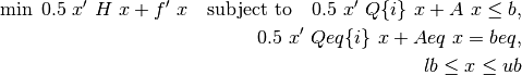
knitro_qcqp
Solve quadratically constrained quadratic programs (or second order cone programs) expressed in the form:
[x,fval,exitflag,output,lambda] = ...
    knitro_qcqp(H,f,Q,A,b,Qeq,Aeq,beq,lb,ub,x0,extendedFeatures,options,knitroOptsFile)
Input Arguments
H: Quadratic objective coefficients represented by an n x n symmetric matrix (where n is the number of variables).
f: Linear objective coefficients.
Q: Quadratic coefficients for inequality constraints. Q is a cell array whose elements (one for each inequality constraint) are n x n symmetric matrices (where n is the number of variables). For Q{i} =[] the constraint reduces to a linear inequality.
A: Coefficient matrix for linear terms in inequality constraints.
b: Upper bound vector for inequality constraints.
Qeq: Quadratic coefficients for equality constraints. Qeq is a cell array whose elements (one for each equality constraint) are n x n symmetric matrices (where n is the number of variables). For Qeq{i} =[] the constraint reduces to a linear equality (optional).
Aeq: Coefficient matrix for linear terms in equality constraints (optional).
beq: Right-hand side vector for equality constraints (optional).
lb: Variable lower bound vector (optional).
ub: Variable upper bound vector (optional).
x0: Initial point vector (optional).
extendedFeatures: Structure used to input additional model features, see The extendedFeatures Structure (optional).
options: Knitro options structure generated from knitro_options, see knitro_options (optional),
knitroOptsFile: Knitro options filename used to set Knitro options specified in a text file, see Setting options (optional).
Only the first two arguments are required. An empty argument can be specified using [].
Output Arguments
x: The optimal solution vector.
fval: The optimal solution objective value.
exitflag: Integer identifying the reason for termination of the algorithm.
output: Structure containing solution information about the optimization.
lambda: Structure containing the Lagrange multipliers at the solution with a different field for each constraint type.
Only the first output argument is required. An empty argument can be specified using [].
knitro_qp
Solve quadratic programs expressed in the form:

[x,fval,exitflag,output,lambda] = ...
    knitro_qp(H,f,A,b,Aeq,beq,lb,ub,x0,extendedFeatures,options,knitroOptsFile)
Input Arguments
H: Quadratic objective coefficients represented by an n x n symmetric matrix (where n is the number of variables).
f: Linear objective coefficients.
A: Coefficient matrix for linear inequality constraints.
b: Upper bound vector for linear inequality constraints.
Aeq: Coefficient matrix for linear equality constraints (optional).
beq: Right-hand side vector for linear equality constraints (optional).
lb: Variable lower bound vector (optional).
ub: Variable upper bound vector (optional).
x0: Initial point vector (optional).
extendedFeatures: Structure used to input additional model features, see The extendedFeatures Structure (optional).
options: Knitro options structure generated from knitro_options, see knitro_options (optional),
knitroOptsFile: Knitro options filename used to set Knitro options specified in a text file, see Setting options (optional).
Only the first two arguments are required. An empty argument can be specified using [].
Output Arguments
x: The optimal solution vector.
fval: The optimal solution objective value.
exitflag: Integer identifying the reason for termination of the algorithm.
output: Structure containing solution information about the optimization.
lambda: Structure containing the Lagrange multipliers at the solution with a different field for each constraint type.
Only the first output argument is required. An empty argument can be specified using [].
knitro_solve
Solve any optimization, nonlinear equations or nonlinear least-squares model defined using the “problem-based” MATLAB API:
[x,fval,exitflag,output,lambda] = ...
    knitro_solve(prob,x0,extendedFeatures,options,knitroOptsFile)
Input Arguments
prob: A problem object created via the MATLAB “problem-based” approach for defining optimization problems.
x0: Initial point vector (optional).
extendedFeatures: Structure used to input additional model features, see The extendedFeatures Structure (optional).
options: Knitro options structure generated from knitro_options, see knitro_options (optional),
knitroOptsFile: Knitro options filename used to set Knitro options specified in a text file, see Setting options (optional).
Only the first argument is required. An empty argument can be specified using [].
Output Arguments
x: The optimal solution vector.
fval: The optimal solution objective value.
exitflag: Integer identifying the reason for termination of the algorithm.
output: Structure containing solution information about the optimization.
lambda: Structure containing the Lagrange multipliers at the solution with a different field for each constraint type.
Only the first output argument is required. An empty argument can be specified using [].
The extendedFeatures Structure
The extendedFeatures structure can be used to define other, extended modeling features of Knitro when using the Knitro/MATLAB interface.
Currently it is used for complementarity constraints, the output function, parallel finite differencing, initial lambda values, custom finite-difference step sizes, custom feasibility tolerances, custom scalings, custom treatments of integer variables, specification of linear variables, custom setting of honor bounds, and some Hessian and Jacobian information. The possible fields for the extendedFeatures structure are described below.
Fields
ccIndexList1 and ccIndexList2: These two complementarity constraint fields may be used to specify the variable index lists for variables complementary to each other. The same index may not appear more than once in the lists.
lambdaInitial: This field allows the user to specify the initial lambda values in a structure with a different field for each constraint type. The fields are ineqlin for linear inequality constraints, eqlin for linear equality constraints, ineqnonlin for nonlinear inequality constraints, eqnonlin for nonlinear equality constraints, upper for upper bounds of variables, and lower for lower bounds of variables. If only some of the fields are defined, the missing fields will be filled with zeros. If none of the fields are defined, Knitro will compute an initial value.
FinDiffRelStep: This field can be used to specify custom step size values for finite-differencing.
LinearVars: This field can be used to specify which variables in the model only appear linearly in the objective and constraints. This information can then be used to perform additional presolve operations. See
KN_set_var_properties()for more details.HonorBnds: This field can be used to specify which variables in the model must satisfy their bounds throughout the optimization. See
KN_set_var_honorbnds()for more details.AFeasTols, AeqFeasTols, cFeasTols, ceqFeasTols, and xFeasTols: These fields can be used to specify custom feasibility tolerances for problem constraints and variables. See
KN_set_con_feastols()andKN_set_var_feastols()for more details.AScaleFactors, AeqScaleFactors, cScaleFactors, ceqScaleFactors, xScaleFactors, xScaleCenters, and objScaleFactor: These fields can be used to specify custom scalings for problem constraints, variables, and the objective. See
KN_set_con_scalings(),KN_set_var_scalings()andKN_set_obj_scaling()for details on how these scalings should be defined.xIntStrategy: This field can be used to specify customized treatments for integer variables. See
KN_set_mip_intvar_strategies()for more details.The other six available fields are JacobPattern, HessPattern, HessFcn, HessMult, OutputFcn, and UseParallel. They have the same properties as the options set by optimset.
Passing Function Arguments
The objective function, fun, can be specified as a function handle for a MATLAB function, as in
x = knitro_nlp(@objFunc,x0)
with a function
function [f,g] = objFunc(x)
    f = x^2;
    g = 2*x;
or as a function handle for an anonymous function:
x = knitro_nlp(@(x)x^2,x0)
The constraint function, nonlcon, is similar, but it returns at least two vectors, c and ceq. It may additionally return two matrices, the gradient matrix of the nonlinear inequality constraints, and the gradient matrix of the nonlinear equality constraints. The third and fourth arguments are only needed when gradopt is set to 1.
Output Structure Fields
Output Argument |
Field |
Description |
|---|---|---|
output |
iterations |
Number of iterations. |
output |
funcCount |
Number of function evaluations. |
output |
constrviolation |
Maximum of constraint violations. |
output |
firstorderopt |
Measure of first-order optimality. |
lambda |
lower |
Lower bounds |
lambda |
upper |
Upper bounds |
lambda |
ineqlin |
Linear inequalities |
lambda |
eqlin |
Linear equalities |
lambda |
ineqnonlin |
Nonlinear inequalities |
lambda |
eqnonlin |
Nonlinear equalities |
Setting Options
The Knitro/MATLAB interface functions take up to two options inputs. The first is an options structure generated from the knitro_options function (see knitro_options). This structure is similar in form to the one passed to the MATLAB function fmincon, using optimset or optimoptions, but uses Knitro-specific option names. It also accepts the MATLAB UseParallel option name.
Here you pass a set of Knitro-specific option names and numeric values to knitro_options and it returns an options structure that can be passed in to any of the Knitro/MATLAB optimization functions. For a complete list of Knitro options and their corresponding numeric options values, see Knitro user options. The example above shows how to set options using the options structure generated from knitro_options.
Options Structure Example:
options = knitro_options('nlp_algorithm', 1, 'outlev', 4 , 'gradopt', 1, ...
                         'hessopt', 1, 'maxit', 1000, 'xtol', 1e-15, ...
                         'feastol', 1e-8, 'opttol', 1e-8, ...
                         'bar_maxcrossit', 5);
[x,fval,exitflag,output,lambda,grad,hess] = ...
        knitro_nlp(@objfun,x0,A,b,Aeq,beq,lb,ub,@constfun,extendedFeatures,options);
The second way to pass Knitro options is to use a Knitro options text file. This is a simple text file where each line contains an option name and value separated by whitespace. Comments beginning with the # sign are ignored and empty lines are ignored. To use this approach, create an options text file as described for the callable library, and include the file as the last argument in the call to the appropriate Knitro/MATLAB interface function.
Settings from the Knitro options text file and the extendedFeatures structure will take precedence over settings made through a knitro_options options structure. Also, note that when using a Knitro options file, option values can be specified either as numeric values or using string values (where appropriate), whereas only numeric values are currently allowed in the setting of an options structure using knitro_options.
The example below shows how to set options using a Knitro options text file called knitro.opt.
Options File Example:
[x,fval,exitflag,output,lambda,grad,hess] = ...
        knitro_nlp(@objfun,x0,A,b,Aeq,beq,lb,ub,@constfun,extendedFeatures,[], ...
        'knitro.opt');
knitro.opt:
nlp_algorithm direct    # Equivalent to setting 'Algorithm' to 'interior-point'
outlev iter_verbose # Equivalent to setting 'Display' to 'iter'
gradopt exact       # Equivalent to setting 'GradObj' to 'on' and 'GradConstr' to 'on'
hessopt exact       # Equivalent to setting 'Hessian' to 'on'
maxit 1000          # Equivalent to setting 'MaxIter' to 1000
xtol 1e-15          # Equivalent to setting 'TolX' to 1e-15
feastol 1e-8        # Equivalent to setting 'TolCon' to 1e-8
opttol 1e-8         # Equivalent to setting 'TolFun' to 1e-8
bar_maxcrossit 5    # Allow a maximum of 5 crossover iterations
Parallelism
There are two types of parallelism that can be used in Knitro/MATLAB. The first is parallel finite-differencing. Parallel finite-differencing is specified in Knitro/MATLAB using the MATLAB UseParallel option and this parallelism occurs at the MATLAB level. The UseParallel option can be specified either through the knitro_options function or using the extendedFeatures structure. It has no effect when exact/user-supplied gradients are used or if the Parallel Computing Toolbox is not installed. The MATLAB command “parpool(n)” will set the number of workers to the minimum of n and the maximum number allowed, which can be set in the cluster profile. If the parallel pool is not started before Knitro is run, it will start one with the default number of workers set by MATLAB, as long as the Parallel Pool preferences allow automatically creating a parallel pool.
The second type of parallelism that can be specified in Knitro/MATLAB is parallelism internal to the Knitro solver mainly related to linear algebra operation used inside Knitro. This type of parallelism is specified using the Knitro option numthreads, which can be set either using the knitro_options function or using a Knitro options text file. The Knitro option “numthreads” does not have an effect on parallel finite-differencing.
Note that some Knitro parallel features that require running multiple Knitro solves in parallel (such as parallel multi-start, parallel algorithms and the parallel Tuner) cannot be used or are ineffective through the Knitro/MATLAB interface because of thread-safety issues specific to the MATLAB Mex interface environment.
Output Function
The output function can be assigned with
extendedFeatures.OutputFcn = @outputfun;
or in the options structure with
options = optimset('OutputFcn',@outputfun);
where the function is defined as
function stop = outputfun(x,optimValues,state);
Only the value of stop can be set to true or false. Setting it to true will terminate Knitro.
The inputs to the function cannot be modified. The inputs include the current point x, the structure optimValues, and the state. Since Knitro only calls the function after every iteration, the value of state will always be ‘iter’. The optimValues structure contains the following fields:
optimValues Fields
optimValues Field |
Description |
|---|---|
lambda |
Structure containing the Lagrange multipliers at the solution with a different field for each constraint type. |
fval |
The objective value at x. |
c |
The nonlinear inequality constraint values at x. |
ceq |
The nonlinear equality constraint values at x. |
gradient |
The gradient vector at x. |
cineqjac |
The nonlinear inequality constraint Jacobian matrix. |
ceqjac |
The nonlinear equality constraint Jacobian matrix. |
Note that setting newpoint to any value other than 3 in the Knitro options file will take precedence over OutputFcn. Note that the nonlinear constraint Jacobian matrices are given with the variables as the rows and constraints as the columns, the transpose of JacobPattern.
Sparsity Pattern for Nonlinear Constraints
The sparsity pattern for the constraint Jacobian is a matrix, which is passed as the JacobPattern option. JacobPattern is only for the nonlinear constraints, with one row for each constraint. The nonlinear inequalities, in order, make up the first rows, and the nonlinear equalities, in order, are in the rows after that. Gradients for linear constraints are not included in this matrix, since the sparsity pattern is known from the linear coefficient matrices.
All that matters for the matrix is whether the values are zero or not zero for each entry. A nonzero value indicates that a value is expected from the gradient function. A MATLAB sparse matrix may be used, which may be more efficient for large sparse matrices of constraints.
The gradients of the constraints returned by the nonlinear constraint function and those used in the newpoint function have the transpose of the Jacobian pattern, i.e., JacobPattern has a row for each nonlinear constraint and a column for each variable, while the gradient matrices (one for inequalities and one for equalities) have a column for each constraint and a row for each variable.
Hessians
The Hessian is the matrix of the second derivative of the Lagrangian, as in
http://www.mathworks.com/help/optim/ug/fmincon.html#brh002z
The matrix H can be given as a full or sparse matrix of the upper triangular or whole matrix pattern.
If HessMult is used, then the Hessian-vector-product of the Hessian and a vector supplied by Knitro at that iteration is returned.
Return codes / exit flags
The returned exit flags will correspond with Knitro’s return code, rather than matching fmincon’s exit flags.
Upon completion, Knitro displays a message and returns an exit code to MATLAB. In the example above Knitro found a solution, so the message was:
Locally optimal solution found
with the return value of exitflag set to 0.
If a solution is not found, then Knitro returns one of the following:
Value |
Description |
|---|---|
0 |
Locally optimal solution found. |
-100 |
Current feasible solution estimate cannot be improved. Nearly optimal. |
-101 |
Relative change in feasible solution estimate < xtol. |
-102 |
Current feasible solution estimate cannot be improved. |
-103 |
Relative change in feasible objective < ftol for ftol_iters. |
-104 |
Returning best feasible iterate (when |
-105 |
Multistart: Feasible point found. |
-200 |
Convergence to an infeasible point. Problem may be locally infeasible. |
-201 |
Relative change in infeasible solution estimate < xtol. |
-202 |
Current infeasible solution estimate cannot be improved. |
-203 |
Multistart: No primal feasible point found. |
-204 |
Problem determined to be infeasible with respect to constraint bounds. |
-205 |
Problem determined to be infeasible with respect to variable bounds. |
-300 |
Problem appears to be unbounded. |
-400 |
Iteration limit reached. Current point is feasible. |
-401 |
Time limit reached. Current point is feasible. |
-402 |
Function evaluation limit reached. Current point is feasible. |
-403 |
MIP: All nodes have been explored. Integer feasible point found. |
-404 |
MIP: Integer feasible point found. |
-405 |
MIP: Subproblem solve limit reached. Integer feasible point found. |
-406 |
MIP: Node limit reached. Integer feasible point found. |
-410 |
Iteration limit reached. Current point is infeasible. |
-411 |
Time limit reached. Current point is infeasible. |
-412 |
Function evaluation limit reached. Current point is infeasible. |
-413 |
MIP: All nodes have been explored. No integer feasible point found. |
-415 |
MIP: Subproblem solve limit reached. No integer feasible point found. |
-416 |
MIP: Node limit reached. No integer feasible point found. |
-501 |
LP solver error. |
-502 |
Evaluation error. |
-503 |
Not enough memory. |
-504 |
Terminated by user. |
-505 to -522 |
Input or other API error. |
-523 |
Derivative check failed. |
-524 |
Derivative check finished. |
-600 |
Internal Knitro error. |
For more information on return codes, see Return codes.